- MIMIC models (with formative and reflective manifest variables connected to a latent construct)
- Confirmatory factor analysis with both continuous and ordinal data
- Linear Algebra
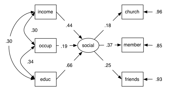
MIMIC Model
Contributed by tim.bates@ed.ac.uk, any errors or questions, please post on the forums.
This is an example from chapter 13 of Schumacker and Lomax's Beginner's guide to SEM
The fitted model is as follows:

Not shown on this diagram is the fact that the variance of the formative variables (income, occupation, education) are fixed to 1 (the data input are a correlation matrix) (hat-tip to Andreas Brandmaier for this!)
require(sem) require(OpenMx) # Often you will see data presented as a lower diagonal. # the readMoments() function in the sem package is a nice helper to read this from the screen: data = sem::readMoments(file = "", diag = TRUE) 1 .304 1 .305 .344 1 .100 .156 .158 1 .284 .192 .324 .360 1 .176 .136 .226 .210 .265 1 # terminates with an empty line: see ?readMoments for more help # now lets fill in the upper triangle with a flipped version of the lower data[upper.tri(data, diag=F)] = t(data)[upper.tri(data, diag=F)] # Set up manifest variables manifests = c("income", "occup", "educ", "church", "member", "friends") # Use these to create names for our dataframe dimnames(data) = list(manifests, manifests) # And latents latents = "social" # 1 latent, with three formative inputs, and three reflective outputs (each with residuals) # Just to be helpful to myself, I've made lists of the formative sources, and the reflective receiver variables in this MIMIC model receivers = manifests[4:6] sources = manifests[1:3] MIMIC <- mxModel("MIMIC", type="RAM", manifestVars = manifests, latentVars = latents, # Factor loadings mxPath(from = sources , to = "social" ), mxPath(from = "social", to = receivers), # Correlated formative sources for F1, each with variance = 1 mxPath(from = sources, connect = "unique.bivariate", arrows = 2), mxPath(from = sources, arrows = 2, values = 1, free=F ), # Residual variance on receivers mxPath(from = receivers, arrows = 2), mxData(data, type = "cov", numObs = 530) ) MIMIC <- mxRun(MIMIC); summary(MIMIC)
  free parameters:
     name matrix     row     col   Estimate   Std.Error lbound ubound
  1        A  social  income 0.13244947  5.51420454
  2        A  social   occup 0.05701774  2.37389629
  3        A  social    educ 0.19511219  8.12304135
  4        A  church  social 0.60971866 25.38489597
  5        A  member  social 1.28671307 53.56883563
  6        A friends  social 0.86519046 36.02017596
  7        S  income   occup 0.30399991  0.03764547
  8        S  income    educ 0.30499977  0.03761111
  9        S   occup    educ 0.34399974  0.03618180
  10       S  church  church 0.96770471  0.05954356
  11       S  member  member 0.85617184  0.05267749
  12       S friends friends 0.93497178  0.05749125

  observed statistics:  21
  estimated parameters:  12
  degrees of freedom:  9
  -2 log likelihood:  2893.752
  saturated -2 log likelihood:  2804.686
  number of observations:  530
  chi-square:  89.06589
  p:  2.506216e-15
  Information Criteria:
      df Penalty Parameters Penalty Sample-Size Adjusted
  AIC   71.06589           113.0659                   NA
  BIC   32.61000           164.3404              126.249
  CFI: 0.7740255
  TLI: 0.6233758
  RMSEA:  0.1295581
Joint continuous and ordinal CFA
Contributed by tim.bates@ed.ac.uk, any errors or questions, please post on the forums.
Data: Built-in example data frame
Variables: One continuous variable, and two binary ordinal variables
require(OpenMx) require(psych) # Read in an example dataset supplied with the OpenMx package data(myFADataRaw) # Grab three variables df <- myFADataRaw[, c("x1","z1", "z3")] # rename them to be more memorable manifests = c("cont1", "ord1","ord2") names(df) <-manifests # For OpenMx to work with ordinal data, they must be ordered factors! df$ord1 <- mxFactor(df$ord1, levels=0:1) df$ord2 <- mxFactor(df$ord2, levels=0:2) # Let's see what we're working with now str(df) 'data.frame': 500 obs. of 3 variables: $ cont1: num 1 1.63 1.95 2.95 3.66 ... $ ord1 : Ord.factor w/ 2 levels "0"<"1": 2 2 2 2 2 2 2 2 2 1 ... $ ord2 : Ord.factor w/ 3 levels "0"<"1"<"2": 1 2 2 1 2 2 1 2 1 1 ... hist(df$cont1) # nice and normal plot(~df$ord1) # binary - 4x as many 1s as 0s plot(~df$ord2) # three-values: low endorsement of the highest value # Just to help keep things simple in the model, let's list up the continuous # and the ordinal manifests separately ordinalVars = manifests[2:3] continuousVars = manifests[1] m1 <- mxModel("joint CFA", type="RAM", manifestVars = manifests, latentVars = "F1", # Factor loadings mxPath(from="F1", to = manifests, arrows=1, free=T, values=1, labels=c("l1","l2","l3")), # Manifest continuous mean & residual variance (both free) mxPath(from="one", to = continuousVars, arrows=1, free=T, values=0, labels="meancont1"), mxPath(from=continuousVars , arrows=2, free=T, values=1, labels="e1" ), # Ordinal manifests mean and variance fixed at 0 & 1 # The thresholds will be computed as being based off this underlying normal distribution) mxPath(from="one", to = ordinalVars, arrows=1, free=F, values=0, labels=c("meanord1","meanord2")), mxPath(from=ordinalVars , arrows=2, free=F, values=1, labels=c("e2","e3")), # fix latent variable variance @1 & mean @0 mxPath(from="F1" , arrows=2, free=F, values=1, labels ="varF1"), mxPath(from="one", to="F1", arrows=1, free=F, values=0, labels="meanF1"), # Make a matrix as wide as the number of ordinal variables (2), and as many rows as the max # of thresholds (3) - 1 # In this case that is 2 * 2 # leave it free where there is a real threshold to be set, and fill the rest of each column fixed @NA # set the column names to the name of the ordinal variables: that is how OpenMx maps into this threshold matrix mxMatrix("Full", nrow=2, ncol=2, byrow=T, name="thresh", dimnames = list(c(), ordinalVars), free = c(T, T , F, T), values = c(0, -1, NA, 1) ), # Add some data mxData(df, type="raw"), # tell the mxRAMObjective that we have not only A,S, F and M matrices, but also some ordinal vars with thresholds mxRAMObjective(A="A", S="S", F="F", M="M", thresholds="thresh") ) # run! m1 = mxRun(m1); summary(m1) free parameters: name matrix row col Estimate Std.Error lbound ubound 1 l1 A cont1 F1 -0.1953311 0.04115263 2 l2 A ord1 F1 -1.0135426 NaN 3 l3 A ord2 F1 -4.3049347 NaN 4 e1 S cont1 cont1 0.9571266 0.06018277 5 meancont1 M 1 cont1 2.9876221 0.04461568 6
| Attachment | Size |
|---|---|
| MIMIC.png | 29.38 KB |
| MIMIC.R | 4.03 KB |
| joint_ordinal_CFA.R | 3.75 KB |
