

| Attachment | Size |
|---|---|
| 13.71 KB | |
| 542 bytes | |
| 547 bytes |
Dear Cheung,
First of all, thank you for your helpful and inspiring contribution. We are very grateful for your interesting work and now we are trying to follow your steps and conduct a meta-analysis. However, on the way, we have had some doubts that we wanted to share with you as we are looking for some advice.
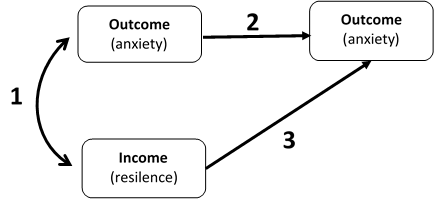
We conducted a data collection of the correlations between an income and longitudinal outcome. Let's imagine, resilence as income and anxiety as outcome. That is, we collected three correlations per study and the time elapsed between waves. When we calculated the degrees of freedom (DF) of the model, we supposed that elapsed time would increase the DF.
We run the model using the code displayed below and we found convergence in some cases (some combinations of incomes/outcomes/population), while in other cases unfortunately the model failed to converge even using rerun(). Additionally, we realized that our model had not enough degrees of freedom to estimate the fit indices.
Our doubts are the following:
- Apart from rerun() function, is there any way or method to get convergence in OSMASEM?
- have you got any recommendation for cases in which there are not enough degrees of freedom to estimate fit indices? Is it a usual practice to publish the results without fit indices in this type of methodologies? In connection with this, have you got any idea on how to deal with the lack of fit indices when reporting data in a paper?
Thank you very much in advance,
best regards.
NOTE: I attach a data frame with convergence (converged.dat) and without convergence (non-converged.dat). Both document are .RData (not allowed by this forum). But I have saved as .dat.
The code:
load("non-converged.dat")
#load("converged.dat")
data <- datos$data
n <- datos$n$N2
lag<-datos$lag$Tiempo

my.df <- Cor2DataFrame(data, n, acov = "weighted")
my.df$data <- data.frame(my.df$data, Lag=scale(lag),
                         check.names=FALSE)
pattern.na(my.df, show.na=FALSE, type="osmasem")

model1 <- 'O2 ~ o1o2*O1 + i102*I1
           I1 ~~ i1WITHo1*O1
           I1 ~~ 1*I1
           O1 ~~ 1*O1
           O2 ~~ Errs2*O2'

RAM1 <- lavaan2RAM(model1, obs.variables=c("O1", "I1", "O2"))

Ax <- matrix(c(0,0,0,
               0,0,0,
               "0*data.Lag","0*data.Lag",0),
             nrow=3, ncol=3, byrow=TRUE)
fit<-osmasem(model.name="Ax as moderator",RAM=RAM1,Ax=Ax, data=my.df)
fitSum<-summary(fit,fitIndices=TRUE)
fit<-rerun(fit, autofixtau2=TRUE)
fitSum<-summary(fit)
fitSum
The output:
free parameters:
      name  matrix row col     Estimate Std.Error A       z value  Pr(>|z|)
1     o1o2      A0  O2  O1   0.72942797 61.868395    0.0117899935 0.9905932
2     i102      A0  O2  I1   0.08720208 67.308102    0.0012955659 0.9989663
3 i1WITHo1      S0  I1  O1  -0.24744425 50.713200   -0.0048792868 0.9961069
4   o1o2_1      A1  O2  O1   0.03189127 56.278375    0.0005666701 0.9995479
5   i102_1      A1  O2  I1  -0.06617169 60.655999   -0.0010909340 0.9991296
6   Tau1_1 vecTau1   1   1 -22.14979597        NA !            NA        NA
7   Tau1_2 vecTau1   2   1  -3.07424264  3.032155   -1.0138804284 0.3106398
8   Tau1_3 vecTau1   3   1 -84.96040254        NA !            NA        NA

Model Statistics:
               |  Parameters  |  Degrees of Freedom  |  Fit (-2lnL units)
       Model:              8                     10             -32.15276
   Saturated:              9                      9                    NA
Independence:              6                     12                    NA
Number of observations/statistics: 556/18

Information Criteria:
      |  df Penalty  |  Parameters Penalty  |  Sample-Size Adjusted
AIC:      -52.15276              -16.15276               -15.889510
BIC:      -95.36045               18.41338                -6.982323
To get additional fit indices, see help(mxRefModels)
timestamp: 2021-03-25 17:06:22
Wall clock time: 0.1089311 secs
OpenMx version number: 2.17.4
Need help?  See help(mxSummary)