Genetic Epidemiology, Path Specification
Mx is probably most popular statistical modeling package in the behavior genetics field, as it was conceived with genetic models in mind, which rely heavily on multiple groups. We introduce here an OpenMx script for the basic genetic model in genetic epidemiologic research, the ACE model. This model assumes that the variability in a phenotype, or observed variable, can be explained by differences in genetic and environmental factors, with A representing additive genetic factors, C shared/common environmental factors and E unique/specific environmental factors (see Neale & Cardon 1992, for a detailed treatment). To estimate these three sources of variance, data have to be collected on relatives with different levels of genetic and environmental similarity to provide sufficient information to identify the parameters. One such design is the classical twin study, which compares the similarity of identical (monozygotic, MZ) and fraternal (dizygotic, DZ) twins to infer the role of A, C and E.
The example starts with the ACE model and includes one submodel, the AE model. It is available in the following file:
A parallel version of this example, using matrix specification of models rather than paths, can be found here:
ACE Model: a Twin Analysis
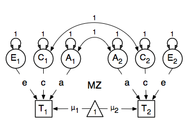
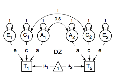
A twin analysis is a typical example of multiple groups, in this case MZ twins and DZ twins, with different expectations for the covariance structure (and possibly means). We illustrate the model here with the corresponding two path diagrams:
Data
Let us assume you have collected data on a large sample of twin pairs for your phenotype of interest. For illustration purposes, we use Australian data on body mass index (BMI) which are saved in a text file ‘myTwinData.txt’. We use R to read the data into a data.frame and to create two subsets of the data for MZ females (mzData) and DZ females (dzData) respectively with the code below. We also define the objects selVars for the variables selected for analysis, and aceVars for the latent variables to simplify the OpenMx code.
require(OpenMx)

#Prepare Data
data(myTwinData)
twinVars <- c(  'fam','age','zyg','part',
                'wt1','wt2','ht1','ht2','htwt1','htwt2','bmi1','bmi2')
summary(myTwinData)
selVars <- c('bmi1','bmi2')
aceVars <- c("A1","C1","E1","A2","C2","E2")
mzData <- as.matrix(subset(myTwinData, zyg==1, c(bmi1,bmi2)))
dzData <- as.matrix(subset(myTwinData, zyg==3, c(bmi1,bmi2)))
colMeans(mzData,na.rm=TRUE)
colMeans(dzData,na.rm=TRUE)
cov(mzData,use="complete")
cov(dzData,use="complete")
Model Specification
There are different ways to draw a path diagram of the ACE model. The most commonly used approach is with the three latent variables in circles at the top, separately for twin 1 and twin 2 respectively called A1, C1, E1 and A2, C2, E2. The latent variables are connected to the observed variables in boxes at the bottom, representing the measures for twin 1 and twin 2: T1 and T2, by single-headed arrows from the latent to the manifest variables. Path coefficients a, c and e are estimated but constrained to be the same for twin 1 and twin 2, as well as for MZ and DZ twins. As MZ twins share all their genotypes, the double-headed path connecting A1 and A2 is fixed to one in the MZ diagram. DZ twins share on average half their genes, and as a result the corresponding path is fixed to 0.5 in the DZ diagram. As environmental factors that are shared between twins are assumed to increase similarity between twins to the same extent in MZ and DZ twins (equal environments assumption), the double-headed path connecting C1 and C2 is fixed to one in both diagrams above. The unique environmental factors are by definition uncorrelated between twins.
Let’s go through the paths specification step by step. First, we start with the require(OpenMx) statement. We include the full code here. As MZ and DZ have to be evaluated together, the models for each will be arguments of a bigger model. Given the diagrams for the MZ and the DZ group look rather similar, we start by specifying all the common elements in yet another model, called ACEModel which will then be shared with the two submodels for each of the twin types, defined in separate mxModel commands. The latter two MxModel objects (mzModel and dzModel) are arguments of the overall twinACE model, and will be saved together in the R object twinACEModel and thus be run together.
#Fit ACE Model with RawData and Path-Style Input
ACEModel <- mxModel("ACE",
    type="RAM",
    manifestVars=selVars,
    latentVars=aceVars,
    # variances of latent variables
    mxPath(
        from=aceVars,
        arrows=2,
        free=FALSE,
        values=1
    ),
    # means of latent variables
    mxPath(
        from="one",
        to=aceVars,
        arrows=1,
        free=FALSE,
        values=0
    ),
    # means of observed variables
    mxPath(
        from="one",
        to=selVars,
        arrows=1,
        free=TRUE,
        values=20,
        labels="mean",
    ),
    # path coefficients for twin 1
    mxPath(
        from=c("A1","C1","E1"),
        to="bmi1",
        arrows=1,
        free=TRUE,
        values=.6,
        label=c("a","c","e")
    ),
    # path coefficients for twin 2
    mxPath(
        from=c("A2","C2","E2"),
        to="bmi2",
        arrows=1,
        free=TRUE,
        values=.6,
        label=c("a","c","e")
    ),
    # covariance between C1 & C2
    mxPath(
        from="C1",
        to="C2",
        arrows=2,
        free=FALSE,
        values=1
    )
)
mzModel <- mxModel(ACEModel, name="MZ",
    # covariance between A1 & A2
    mxPath(
        from="A1",
        to="A2",
        arrows=2,
        free=FALSE,
        values=1
    ),
    mxData(
        observed=mzData,
        type="raw"
    )
)
dzModel <- mxModel(ACEModel, name="DZ",
# covariance between A1 & A2
    mxPath(
        from="A1",
        to="A2",
        arrows=2,
        free=FALSE,
        values=.5
    ),
    mxData(
        observed=dzData,
        type="raw"
    )
)
twinACEModel <- mxModel("twinACE", mzModel, dzModel,
    mxAlgebra(
        expression=MZ.objective + DZ.objective,
        name="minus2loglikelihood"
    ),
    mxAlgebraObjective("minus2loglikelihood")
)
Now we will discuss the script line by line. For further details on RAM, see ref. Note that we left the comma’s at the end of the lines which are necessary when all the arguments are combined prior to running the model. Each line can be pasted into R, and then evaluated together once the whole model is specified. Models specifying paths are translated into ‘RAM’ specifications for optimization, indicated by using the type="RAM". We start the path diagram specification by providing the names for the manifest variables in manifestVars and the latent variables in latentVars. We use here the selVars and aceVars objects that we created previously when preparing the data.
mxModel("ACE",
        type="RAM",
        manifestVars=selVars,
        latentVars=aceVars,
We start by specifying paths for the variances and means of the latent variables. These include double-headed arrows from each latent variable back to itself, fixed at one.
# variances of latent variables
mxPath(
    from=aceVars,
    arrows=2,
    free=FALSE,
    values=1
),
and single-headed arrows from the triangle (with a fixed value of one) to each of the latent variables, fixed at zero.
# means of latent variables
mxPath(
    from="one",
    to=aceVars,
    arrows=1,
    free=FALSE,
    values=0
),
Next we specify paths for the means of the observed variables using single-headed arrows from one to each of the manifest variables. These are set to be free and given a start value of 20. As we use the same label (mean) for the two means, they are constrained to be equal. Remember that R ‘recycles’.
# means of observed variables
mxPath(
    from="one",
    to=selVars,
    arrows=1,
    free=TRUE,
    values=20,
    labels="mean"
),
The main paths of interest are those from each of the latent variables to the respective observed variable. These are also estimated (thus all are set free), get a start value of 0.6 and appropriate labels.
# path coefficients for twin 1
mxPath(
    from=c("A1","C1","E1"),
    to="bmi1",
    arrows=1,
    free=TRUE,
    values=0.6,
    label=c("a","c","e")
),
# path coefficients for twin 2
mxPath(
    from=c("A2","C2","E2"),
    to="bmi2",
    arrows=1,
    free=TRUE,
    values=0.6,
    label=c("a","c","e")
),
As the common environmental factors are by definition the same for both twins, we fix the correlation between C1 and C2 to one.
# covariance between C1 & C2
mxPath(
    from="C1",
    to="C2",
    arrows=2,
    free=FALSE,
    values=1
))
We add the paths that are specific to the MZ group or the DZ group into the respective models, mzModel and dzModel, which are combined in twinACEModel. So we have two mxModel statements following the ACEModel model statement. Each of the two models have access to all the paths already defined given ACEModel is the first argument of mzModel and dzModel. In the MZ model we add the path for the correlation between A1 and A2 which is fixed to one. That concludes the specification of the model for the MZ’s, thus we move to the mxData command that calls up the data.frame with the MZ raw data, mzData, with the type specified explicitly. We also give the model a name, MZ, to refer back to it later when we need to add the objective functions.
mzModel <- mxModel(ACEModel, name="MZ",
    # covariance between A1 & A2 in MZ's
    mxPath(
        from="A1",
        to="A2",
        arrows=2,
        free=FALSE,
        values=1
    ),
    mxData(
        observed=mzData,
        type="raw"
    )
)
The mxModel command for the DZ group is very similar, except that the the correlation between A1 and A2 is fixed to 0.5 and the DZ data, dzData are read in, and the model is named DZ. Note that OpenMx can handle constants in algebra.
dzModel <- mxModel(ACEModel, name="DZ",
    # covariance between A1 & A2 in DZ's
    mxPath(
        from="A1",
        to="A2",
        arrows=2,
        free=FALSE,
        values=.5
    ),
    mxData(
        observed=dzData,
        type="raw"
    )
)
Finally, both models need to be evaluated simultaneously. We specify a new mxModel which has the mzModel and dzModel as its arguments. We then generate the sum of the objective functions for the two groups, using mxAlgebra, and use the result (minus2loglikelihood) as argument of the mxAlgebraObjective command.
twinACEModel <- mxModel("twinACE", mzModel, dzModel,
    mxAlgebra(
        expression=MZ.objective + DZ.objective,
        name="minus2loglikelihood"
    ),
    mxAlgebraObjective("minus2loglikelihood")
)
Model Fitting
We need to invoke the mxRun command to start the model evaluation and optimization. Detailed output will be available in the resulting object, which can be obtained by a print() statement.
#Run ACE model
twinACEFit <- mxRun(twinACEModel)
Often, however, one is interested in specific parts of the output. In the case of twin modeling, we typically will inspect the likelihood, the expected covariance matrices and mean vectors, the parameter estimates, and possibly some derived quantities, such as the standardized variance components, obtained by dividing each of the components by the total variance. Note in the code below that the mxEval command allows easy extraction of the values in the various matrices/algebras which form the first argument, with the model name as second argument. Once these values have been put in new objects, we can use any regular R expression to derive further quantities or organize them in a convenient format for including in tables. Note that helper functions could easily (and will likely) be written for standard models to produce ‘standard’ output.
MZc <- twinACEFit$MZ.objective@info$expCov    # expected covariance matrix for MZ's
DZc <- twinACEFit$DZ.objective@info$expCov    # expected covariance matrix for DZ's
M <- twinACEFit$MZ.objective@info$expMean    # expected mean
A <- mxEval(a*a, twinACEFit)    # additive genetic variance, a^2
C <- mxEval(c*c, twinACEFit)    # shared environmental variance, c^2
E <- mxEval(e*e, twinACEFit)    # unique environmental variance, e^2
V <- (A+C+E)    # total variance
a2 <- A/V        # standardized A
c2 <- C/V        # standardized C
e2 <- E/V        # standardized E
ACEest <- rbind(cbind(A,C,E),cbind(a2,c2,e2))    # table of estimates
LL_ACE <- mxEval(objective, twinACEFit)        # likelihood of ACE model
Alternative Models: an AE Model
To evaluate the significance of each of the model parameters, nested submodels are fit in which the parameters of interest are fixed to zero. If the likelihood ratio test between the two models (one including the parameter and the other not) is significant, the parameter that is dropped from the model significantly contributes to the variance of the phenotype in question. Here we show how we can fit the AE model as a submodel with a change in two mxPath commands. First, we define a new model ‘AEModel’ with ‘ACEModel’ as its first argument. ACEModel included the common parts of the model, necessary for both MZ and DZ group. Next we re-specify the path from C1 to bmi1 to be fixed to zero, and do the same for the path from C2 to bmi2. We need to respecify the mzModel and the dzModel, so that they are now built with the changed paths from the common AEModel. We can run this model in the same way as before, by combining the objective functions of the two groups and generate similar summaries of the results.
#Run AE model
AEModel <- mxModel(ACEModel, name="twinAE",
    mxPath(
        from=c("A1","C1","E1"),
        to="bmi1",
        arrows=1,
        free=c(T,F,T),
        values=c(.6,0,.6),
        label=c("a","c","e")
    ),
    mxPath(
        from=c("A2","C2","E2"),
        to="bmi2",
        arrows=1,
        free=c(T,F,T),
        values=c(.6,0,.6),
        label=c("a","c","e")
    )
)
mzModel <- mxModel(AEModel, name="MZ",
    mxPath(
        from="A1",
        to="A2",
        arrows=2,
        free=FALSE,
        values=1
    ),
    mxData(
        observed=mzData,
        type="raw"
    )
)
dzModel <- mxModel(AEModel, name="DZ",
    mxPath(
        from="A1",
        to="A2",
        arrows=2,
        free=FALSE,
        values=.5
    ),
    mxData(
        observed=dzData,
        type="raw"
    )
)
twinAEModel <- mxModel("twinAE", mzModel, dzModel,
    mxAlgebra(
        expression=MZ.objective + DZ.objective,
        name="twin"
    ),
    mxAlgebraObjective("twin")
)

twinAEFit <- mxRun(twinAEModel)


MZc <- twinAEFit$MZ.objective@info$expCov
DZc <- twinAEFit$DZ.objective@info$expCov
M <- twinAEFit$MZ.objective@info$expMean
A <- mxEval(a*a, twinAEFit)
C <- mxEval(c*c, twinAEFit)
E <- mxEval(e*e, twinAEFit)
V <- (A+C+E)
a2 <- A/V
c2 <- C/V
e2 <- E/V
AEest <- rbind(cbind(A, C, E),cbind(a2, c2, e2))
LL_AE <- mxEval(objective, twinAEFit)
We use a likelihood ratio test (or take the difference between -2 times the log-likelihoods of the two models, for the difference in degrees of freedom) to determine the best fitting model, and print relevant output.
LRT_ACE_AE <- LL_AE - LL_ACE

#Print relevant output
ACEest
AEest
LRT_ACE_AE
Note that the way to specify submodels using path specification is not straightforward and requires repeating code. The OpenMx team is currently working on better alternatives. These models may also be specified using matrices instead of paths, which allow for easier submodel specification. See Genetic Epidemiology, Matrix Specification for matrix specification of these models.