
Main menu
You are here
Revision of Example Models from Fri, 03/30/2012 - 09:44
Revisions allow you to track differences between multiple versions of your content, and revert back to older versions.
Main Wiki Page
- MIMIC models (with formative and reflective manifest variables connected to a latent construct)
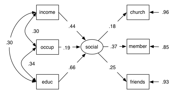
MIMIC Model
This is an example from chapter 13 of Schumacker and Lomax’s Beginner’s guide to SEM
The fitted model is as follows:

mimic model
Not shown on this diagram is the fact that the variance of the formative variables (income, occupation, education) are fixed to 1 (the data input are a correlation matrix) (hat-tip to Andreas Maier for this!)
 require(sem)
 require(OpenMx)

# Often you will see data presented as a lower diagonal.
# the readMoments() function in the sem package is a nice helper to read this from the screen:

data = sem::readMoments(file = "", diag = TRUE)
1
.304 1
.305 .344   1
.100 .156 .158   1
.284 .192 .324 .360   1
.176 .136 .226 .210 .265  1

# terminates with an empty line: see ?readMoments for more help

# now letsfill in the upper triangle with a flipped version of the lower
data[upper.tri(data, diag=F)] = t(data)[upper.tri(data, diag=F)]

# Set up manifest variables
manifests = c("income", "occup", "educ", "church", "member", "friends")

# Use these to create names for our dataframe
dimnames(data) = list(manifests, manifests)

# And latents
latents   = "social" # 1 latent, with three formative inputs, and three reflective outputs (each with residuals)

# Just to be helpful to myself, I've made lists of the formative sources, and the reflective receiver variables in this MIMIC model
receivers = manifests[4:6]
sources   = manifests[1:3]

MIMIC <- mxModel("MIMIC", type="RAM",
    manifestVars = manifests,
    latentVars   = latents,

    # Factor loadings
    mxPath(from = sources , to = "social" , values),
    mxPath(from = "social", to = receivers, values),

    # Correlated formative sources for F1, each with variance = 1
    mxPath(from = sources, connect = "unique.bivariate", arrows = 2),
    mxPath(from = sources, arrows = 2, values = 1, free=F ),

    # Residual variance on receivers
    mxPath(from = receivers, arrows = 2),
    mxData(data, type = "cov", numObs = 530)
)
MIMIC <- mxRun(MIMIC); summary(MIMIC)
  free parameters:
     name matrix     row     col   Estimate   Std.Error lbound ubound
  1        A  social  income 0.13244947  5.51420454
  2        A  social   occup 0.05701774  2.37389629
  3        A  social    educ 0.19511219  8.12304135
  4        A  church  social 0.60971866 25.38489597
  5        A  member  social 1.28671307 53.56883563
  6        A friends  social 0.86519046 36.02017596
  7        S  income   occup 0.30399991  0.03764547
  8        S  income    educ 0.30499977  0.03761111
  9        S   occup    educ 0.34399974  0.03618180
  10       S  church  church 0.96770471  0.05954356
  11       S  member  member 0.85617184  0.05267749
  12       S friends friends 0.93497178  0.05749125

  observed statistics:  21
  estimated parameters:  12
  degrees of freedom:  9
  -2 log likelihood:  2893.752
  saturated -2 log likelihood:  2804.686
  number of observations:  530
  chi-square:  89.06589
  p:  2.506216e-15
  Information Criteria:
      df Penalty Parameters Penalty Sample-Size Adjusted
  AIC   71.06589           113.0659                   NA
  BIC   32.61000           164.3404              126.249
  CFI: 0.7740255
  TLI: 0.6233758
  RMSEA:  0.1295581
- Log in or register to post comments
- Talk
 Printer-friendly version