Item Factor Analysis
What is Item Factor Analysis?
An Intuitive Appeal
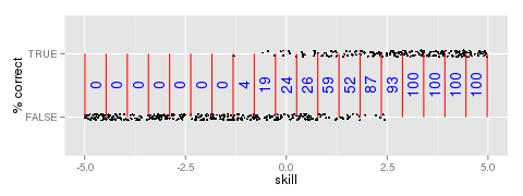
Figure 1: Percentage correct of responses by skill bin
Educational assessments are often scored correct and incorrect. Some items may also offer partial credit for partially correct answers. One approach to analyze these ordinal data is Classical Test Theory (CTT). CTT includes statistics like Cronbach’s α for estimating reliability, proportion correct as an estimate of item difficulty, and item-total correlation as an estimate of item discrimination. However, a disadvantage of CTT is the need for huge samples to establish test norms. Modern Test Theory, also known as Item Response Theory or Item Factor Analysis (IFA), offers substantial advantages over CTT such as the ability to obtain unbiased item parameter estimates from an unrepresentative sample [Embretson1996].
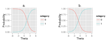
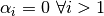
Figure 2: Example plots of the logistic curve
IFA is based on the idea of fitting models to data. The first step
is to convert nominal or ordinal data into interval scale data. To understand how this is
accomplished, assume that the true skill (traditionally  ) of participants is known. We can
plot item outcome by true skill, partition the skill distribution into bins, and count the
proportion of correct responses in each bin (Figure 1). We can fit a model to these data.
One popular model is the logistic model (also called the 1PL or Rasch model),
) of participants is known. We can
plot item outcome by true skill, partition the skill distribution into bins, and count the
proportion of correct responses in each bin (Figure 1). We can fit a model to these data.
One popular model is the logistic model (also called the 1PL or Rasch model),
where is the participant’s skill and c is the estimated parameter to describe the item’s
difficulty (Figure 2). While the examinee’s
true skill is assumed known in this simplified introduction, such an assumption is unnecessary.
There is a circular dependency.
Items parameters depend on examinee skill which, in turn, depend on item parameters.
These kinds of models cannot be optimized directly.
However, optimization is possible by switching back and
forth between item and person parameters [BockAitkin1981].
The Likelihood of Item Models
The best way to appreciate the assumptions involved in Item Factor Analysis is to
examine how the likelihood is traditionally computed.
The conditional likelihood of response  to item
  from person
  with item parameters
  and latent ability
  is
is

One implication of this equation is that items are assumed conditionally independent.
That is, the outcome of one item does not have any influence on
another item after controlling for  and .
The unconditional likelihood is obtained by integrating over
the latent distribution ,
and .
The unconditional likelihood is obtained by integrating over
the latent distribution ,
Typically is distributed as multivariate Normal.
Other distributions are possible, but are not implemented in OpenMx at the time of
this writing.
With an assumption that examinees are independently and identically distributed,
we can sum the individual log likelihoods,
One important observation about this model is that there are two kinds
of parameters.
There are item parameters and latent distribution
parameters .
For didactic purposes,
we will start with models for item parameters and
neglect the latent distribution,
assuming that the latent distribution is standard multivariate Normal.
Once there is some experience with item models,
we will fix item parameters and focus on estimating latent distribution parameters.
Finally, an example will be given of a model that estimates
both item and latent distribution parameters simultaneously.
Item Models
This chapter assumes that you have already read the Basic Introduction.
A Rasch model
Suppose you regularly administer the PANAS [WatsonEtal1988], but instead of scoring participants by adding up the item scores, you want to try IFA. Here is how you might do it. Without loss of generality, we will only consider the positive affect part of the scale.
library(OpenMx)
library(rpf)

PANASItem <- c("Very Slightly or Not at All",  "A Little",
             "Moderately", "Quite a Bit",    "Extremely")
spec <- list()
spec[1:10] <- rpf.grm(outcomes = length(PANASItem))  # grm="graded response model"

# replace with your own data
data <- rpf.sample(750, spec, sapply(spec, rpf.rparam))

for (cx in 1:10) levels(data[[cx]]) <- PANASItem          # repair level labels
colnames(data) <- c("interested", "excited", "strong", "enthusiastic", "proud",
                    "alert", "inspired", "determined", "attentive", "active")
head(data)  # much easier to understand with labels
origData <- data

startingValues <- matrix(c(1, seq(1,-1,length.out=4)), ncol=length(spec), nrow=5)
imat <- mxMatrix(name="item", values=startingValues,
                free=TRUE, dimnames=list(names(rpf.rparam(spec[[1]])), colnames(data)))
rownames(imat)[1] <- "posAff"
imat$labels[1,] <- 'slope'

originalPanas1 <- mxModel(model="panas1", imat,
           mxData(observed=data, type="raw"),
           mxExpectationBA81(ItemSpec=spec, item="item"),
           mxFitFunctionML(),
           mxComputeEM('expectation', 'scores', mxComputeNewtonRaphson()))
panas1 <- mxRun(originalPanas1)
A PANAS item always has 5 possible outcomes, but best practice is to list the outcomes labels and let R count them for you. If you work on a new measure then you will appreciate the ease with which your script can adapt to adding or removing outcomes. Even for PANAS, we could try collapsing two outcomes and see how the model fit changes.
spec <- list()
spec[1:10] <- rpf.grm(outcomes = length(PANASItem))
The rpf.grm function creates an rpf.base class object that represents an item response function. An item response function assigns probabilities to response outcomes. The grm in the function name rpf.grm stands for graded response model. You can inspect the mathematical formula for the graded response model by requesting the manual page with ?rpf.grm. Experiment with the rpf.* functions to get a feel for how they work.
rpf.rparam(spec[[1]])    # generates random parameters
rpf.numParam(spec[[1]])  # same as length(rpf.rparam(spec[[1]]))
rpf.paramInfo(spec[[1]]) # type and default upper & lower bounds
rpf.prob(spec[[1]], startingValues[,1], 0)   # probabilities at score=0
rpf.prob(spec[[1]], startingValues[,1], .5)  # probabilities at score=.5

data <- rpf.sample(750, spec, sapply(spec, rpf.rparam))
This last line (rpf.sample) creates fake data for 750 random participants based on our list of item models and random item parameters. Instead of this line, you would typically read in your data using read.csv and convert it to ordered factors using mxFactor.
startingValues <- matrix(c(1, seq(1,-1,length.out=4)), ncol=length(spec), nrow=5)
We can input particular starting values. That is what we do here. Every column is an item and every row is a different parameter. Regardless of item model, the first rows are factor loadings and the remaining parameters have meanings dependent on the item model. The graded response model is a little finicky; the threshold parameters must be ordered. Alternately, a good way to obtain random starting values is with,
startingValues <- mxSimplify2Array(lapply(spec, rpf.rparam))
startingValues[1,] <- 1  # these parameters must be equal
This is convenient because it will work for a non-homogeneous list of items. There are various circumstances where you will need to fix some of the starting values to particular values. For example:
- To constrain the nominal model to act like the generalized partial credit model
you will set
 .
. - When you have more than 1 factor, you may know a priori that some items do not load on certain factors.
If you need to set some starting values to something specific then you might start with random starting values and then override any rows and columns as needed.
imat <- mxMatrix(name="item", values=startingValues,
                free=TRUE, dimnames=list(names(rpf.rparam(spec[[1]])), colnames(data)))
rownames(imat)[1] <- "posAff"
The item matrix contains response probability function parameters in columns. This layout can be a little awkward when you estimate a mixed format measure with different numbers of outcomes for each item. Fortunately, all the PANAS items are the same. We must label all the rows and columns. The first row must be labeled with the name of our factor, posAff. The remaining rows can take any label. Since all of our items are the same, we can use the default item parameter names. The column names must match the column names of the data.
imat$labels[1,] <- 'slope'
Here we set the label of every parameter in the first row to slope. This is an equality constraint. With this constraint, we assume all items work equally well at measuring the latent trait. This constraint is what makes the difference between a Rasch model and any other kind of IFA model. A Rasch model makes this assumption.
panas1 <- mxModel(model="panas1", imat,
           mxData(observed=data, type="raw"),
           mxExpectationBA81(ItemSpec=spec, item="item"),
           mxFitFunctionML(),
           mxComputeEM('expectation', 'scores', mxComputeNewtonRaphson()))
Here we put everything together. There are a few things that are new.
mxComputeEM('expectation', 'scores', mxComputeNewtonRaphson())
The mxComputeEM plan is a somewhat more sophisticated version of
mxComputeIterate(steps=list(
                 mxComputeOnce('expectation', 'scores'),
                 mxComputeNewtonRaphson(),
                 mxComputeOnce('expectation'),
                 mxComputeOnce('fitfunction', 'fit')))
In both compute plans, OpenMx will iterate until the change in the fitfunction is less than some threshold. For every iteration, person scores are predicted by the expectation, a Newton-Raphson optimization takes place to improve the item parameter values, the predicted person scores are discarded, and the fitfunction is evaluated. In comparison to mxComputeIterate, the mxComputeEM plan offers additional options to speed up convergence and estimate standard errors.
After running the model, we can inspect the parameters estimates,
panas1 <- mxRun(originalPanas1)
panas1$item$values
# or
summary(panas1)
At this point, you might notice something unsettling about the summary output. No standard errors are reported. How do we know whether our model converged? Excellent question. There are a few things that we can check. We can look at the count of EM cycles and M-step Newton-Raphson iterations.
panas1$compute$output
If the number of EM cycles is 2 or less then it is likely that the parameters are still sitting at their starting values. Since our starting values were mostly random, that’s probably not the solution we were looking for. Instead of digging into the MxComputeEM output, we can also re-run the model with extra diagnostics enabled.
panas1 <- mxModel(model=originalPanas1,
               mxComputeEM('expectation', 'scores', mxComputeNewtonRaphson(),
                           verbose=2L))
panas1 <- mxRun(panas1)
Note the addition of verbose=2L to mxComputeEM. The mxComputeNewtonRaphson object takes a verbose parameter as well if you want to examine the progress of the optimization in (much) more detail. From this diagnostic output, we discern that the parameters are changing, but we still do not know whether the solution is a candidate global optimum.
info1 <- mxModel(panas1,
              mxComputeSequence(steps=list(
                mxComputeOnce('fitfunction', 'information', "meat"),
                mxComputeStandardError(),
                mxComputeHessianQuality())))
info1 <- mxRun(info1)
As a starting point, we can estimate the information matrix by taking the inverse of the covariance of the per-row first derivatives. This estimate is called meat because it forms the inside of a sandwich covariance matrix [White1994]. The first thing to look at is the condition number of the information matrix.
info1$output$conditionNumber
A finite condition number implies that the information matrix is positive definite. Since the condition number is roughly closer to zero than to positive infinity, there is a good chance that the parameters are at a candidate global optimum. We can examine the standard errors.
summary(info1)
Further diagnostics are available from the RPF package. Many of these diagnostic functions are most convenient to use when all the relevant information is packaged up into an IFA group object. A convenient way to create an IFA group object is to use as.IFAgroup.
panas1Grp <- as.IFAgroup(panas1)
We know from inspection of the likelihood equation that IFA models assume that items are conditionally independent. That is, the outcome on a given item only depends on its item parameters and examinee skill, not on the outcome of other items. At least some attempt should be made to check this assumption.
ChenThissen1997(panas1Grp)
Item pairs that exhibit statistically significant local dependence and positively correlated residuals should be investigated. If ignored, local dependence exaggerates the accuracy of measurement. Standard errors will be smaller and items will seem to fit the data better than they otherwise would [Yen1993].
Since we have a single factor Rasch model, the residuals are easily interpretable. We can examine Rasch fit statistics infit and outfit. Before we do that, however, we need to compute EAP scores.
panas1Grp$scores <- EAPscores(panas1Grp)

rpf.1dim.fit(group=panas1Grp, margin=2)
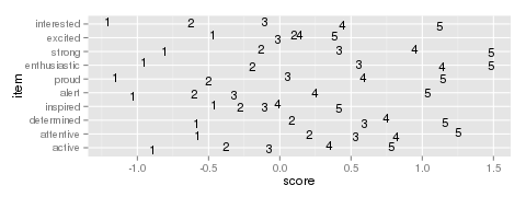
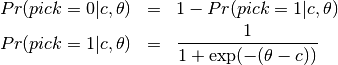
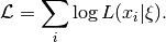
Figure 3: Example item map
This gives us item-wise statistics. For person-wise statistics, we can replace margin=2 with margin=1. For some discussion on the interpretation of these statistics, visit the Infit and Outfit page at the Institute for Objective Measurement. Another way to look at the results is to create an item plot. An item plot assigns to every outcome the mean of the ability of every examinee who picked that outcome (Figure 3).
sumScoreEAP(panas1Grp)
Finally, we can generate a sum-score EAP table. The posAff column contains the interval-scale score corresponding to the row-wise sum-score. You could use this table to score the PANAS instead of merely using the sum-score. The EAP sum-score will likely provide higher accuracy measurement of the latent trait positive affect.
A 2PL model
Suppose you are skeptical that all positive affect items work equally well at measuring positive affect. We can relax this assumption and let the optimizer estimate how well each item is working. Continuing our previous example, all that is needed is to remove the label from the item parameter matrix.
panas2 <- mxModel(model=panas1,
             mxComputeSequence(list(
             mxComputeEM('expectation', 'scores', mxComputeNewtonRaphson()),
             mxComputeOnce('fitfunction', 'information', "meat"),
             mxComputeStandardError(),
             mxComputeHessianQuality())))
panas2$item$labels[1,] <- NA  # here we remove the label
panas2 <- mxRun(panas2)
The compute plan is the same as before except that we combined both the mxComputeEM fit step and computation of standard errors in a single mxComputeSequence. As usual, we start by inspecting the condition number of the Hessian then look at the parameter estimates with standard errors.
panas2$output$conditionNumber
summary(panas2)
Since these models are nested, we can conduct a likelihood ratio test to determine whether panas2 fits the data significantly better than our Rasch constrained model panas1.
mxCompare(panas2, panas1)
Rasch fit statistics are not appropriate for a 2PL model because residuals from different items have different weights. However, we can compare expected item outcome proportions against sum-scores. First we need to create IFA group object for panas2 then we can run the S test [OrlandoThissen2000].
panas2Grp <- as.IFAgroup(panas2)
SitemFit(panas2Grp)
Figure 4: Expected vs observed outcome frequencies at each sum-score level
The internal tables of SitemFit can easily be plotted (Figure 4). Sometimes it is easier to diagnose the source of misfit by examining such a plot than by inspection of large tables of probabilities. However, the S test is not a panacea. Poorly fitting items will cause other items to fit poorly. The S test is just one more tool in the toolbox.
A 3PL with Bayesian priors
The 3PL item model is similar to the 2PL model except with an additional lower asymptote to represent the chance of getting the item correct by guessing. Estimation of 3PL models usually requires very large samples or the use of Bayesian priors on the lower asymptote. For an item with TRUE/FALSE outcomes, the chance of guessing correct is .5. In this case, the mode of the prior would be set to .5. In general, the mode is set to the reciprocal of the number of possible outcomes.
Unlike most other IFA software, OpenMx can accommodate a prior of any form. This flexibility is marvelous, however, it may require some additional effort to set up priors in comparison to other software. Typically the same family of priors would be applied to all asymptote parameters. For didactic purposes, here we will implement a beta prior on half of the asymptote parameters and a Gaussian prior on the remainer.
Asymptote parameters are estimated in logit units.
The advantage of logit units is that there is no
need to complicate the optimization with upper and lower bounds.
To interpret the estimates,
asymptote parameters should be transformed back into
probability units using the logistic function, 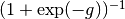 .
.
spec <- list()
spec[1:8] <- rpf.drm()  # drm="dichotomous response model"

# replace with your own data
simParam <- sapply(spec, rpf.rparam)
simParam['u',] <- logit(1)     # fix upper bound at 1 for a 3PL equivalent model
data <- rpf.sample(750, spec, simParam)

imat <- mxMatrix(name="item", values=c(1,0,logit(.1),logit(1)),
                free=c(TRUE, TRUE, TRUE, FALSE), nrow=4, ncol=length(spec),
                dimnames=list(names(rpf.rparam(spec[[1]])), colnames(data)))

# label the pseudo-guessing parameters
imat$labels['g',] <- paste('g',1:length(spec),sep="")

# half of the items get a beta prior
betaRange <- 1:(length(spec)/2)

# the other half get a Gaussian prior
gaussRange <- (1+length(spec)/2):length(spec)

# Create matrices that contain only a subset of the parameters from
# the item matrix so the priors are easier to set up.
betaPrior <- mxMatrix(name="betaPrior", nrow=1, ncol=length(betaRange),
               free=TRUE, labels=imat$labels['g',betaRange],
               values=imat$values['g',betaRange])
gaussPrior <- mxMatrix(name="gaussPrior", nrow=1, ncol=length(gaussRange),
               free=TRUE, labels=imat$labels['g',gaussRange],
               values=imat$values['g',gaussRange])
For beta parameters  and
and  ,
the beta density for logit transformed parameter
,
the beta density for logit transformed parameter  is
is
![\frac{1}{\mathrm{Beta}(\alpha,\beta)} \left[\frac{1}{(1+\exp(-g))}\right]^a \left[1-\frac{1}{1+\exp(-g)}\right]^b.](_images/math/044127bfdffde6e618596f612fecde3c97289ada.png)
After application of  and simplifying, we obtain

and derivatives with respect to are
The mode of the beta density is  and we can regard
 as the informative strength of the prior.
For a given mode and strength, we obtain
as the informative strength of the prior.
For a given mode and strength, we obtain  and
and 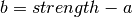 .
It is often helpful to look at a plot (e.g., Figure 5)
to develop your mathematical imagination.
.
It is often helpful to look at a plot (e.g., Figure 5)
to develop your mathematical imagination.
Figure 5: Beta prior of strength 5 with mode logit(1/5) on the logit scale
calcBetaParam <- function(mode, strength) {
  a <- mode * strength
  b <- strength - a
  c(a=a, b=b, c=log(beta(a+1,b+1)))
}

guessChance <- c(1/2, 1/3, 1/4, 1/5)
betaParam <- sapply(guessChance, calcBetaParam, strength=5)

# copy our betaParam table into OpenMx row vectors
betaA <- mxMatrix(name="betaA", nrow=1, ncol=length(betaRange), values=betaParam['a',])
betaB <- mxMatrix(name="betaB", nrow=1, ncol=length(betaRange), values=betaParam['b',])
betaC <- mxMatrix(name="betaC", nrow=1, ncol=length(betaRange), values=betaParam['c',])

# implement the math given above
betaFit <- mxAlgebra(2 * sum((betaA + betaB)*log(exp(betaPrior)+1) -
             betaA * betaPrior + betaC), name="betaFit")
betaGrad <- mxAlgebra(2*(betaB-(betaA+betaB) / (exp(betaPrior) + 1)),
             name="betaGrad", dimnames=list(c(),betaPrior$labels))
betaHess <- mxAlgebra(vec2diag(2*exp(betaPrior)*(betaA+betaB) / (exp(betaPrior) + 1)^2), name="betaHess",
             dimnames=list(betaPrior$labels, betaPrior$labels))

# Create a model that will evaluate to the log likelihood of the beta prior
# and provide suitable derivatives for the optimizer.
betaModel <- mxModel(model="betaModel", betaPrior, betaA, betaB, betaC,
             betaFit, betaGrad, betaHess,
             mxFitFunctionAlgebra("betaFit", gradient="betaGrad", hessian="betaHess"))
In comparison to a beta prior, a Gaussian prior is somewhat easier to set up. A rationale for use of the Gaussian is given in [CaiYangHansen2011]. The mean of the prior is set to the desired mode and the standard deviation can be regarded as the strength of the prior. A standard deviation of 0.5 was suggested by [CaiYangHansen2011].
# These are the prior parameter row vectors.
gaussM <- mxMatrix(name="gaussM", nrow=1, ncol=length(gaussRange), values=logit(guessChance))
gaussSD <- mxMatrix(name="gaussSD", nrow=1, ncol=length(gaussRange), values=.5)

# The single variable Gaussian density and derivatives are well known mathematical results.
gaussFit <- mxAlgebra(sum(log(2*pi) + 2*log(gaussSD) +
             (gaussPrior-gaussM)^2/gaussSD^2), name="gaussFit")
gaussGrad <- mxAlgebra(2*(gaussPrior - gaussM)/gaussSD^2, name="gaussGrad",
             dimnames=list(c(),gaussPrior$labels))
gaussHess <- mxAlgebra(vec2diag(2/gaussSD^2), name="gaussHess",
                   dimnames=list(gaussPrior$labels, gaussPrior$labels))

# Create a model that will evaluate to the log likelihood of the Gaussian prior
# and provide suitable derivatives for the optimizer.
gaussModel <- mxModel(model="gaussModel", gaussPrior, gaussM, gaussSD,
                  gaussFit, gaussGrad, gaussHess,
                  mxFitFunctionAlgebra("gaussFit", gradient="gaussGrad", hessian="gaussHess"))

itemModel <- mxModel(model="itemModel", imat,
           mxData(observed=data, type="raw"),
           mxExpectationBA81(spec),
           mxFitFunctionML())

demo3pl <- mxModel(model="demo3pl", itemModel, betaModel, gaussModel,
                 mxFitFunctionMultigroup(groups=c('itemModel.fitfunction', 'betaModel.fitfunction',
                   'gaussModel.fitfunction')),
                 mxComputeSequence(list(
                   mxComputeEM('itemModel.expectation', 'scores', mxComputeNewtonRaphson()),
                   mxComputeNumericDeriv(),
                   mxComputeHessianQuality(),
                   mxComputeStandardError()
                 )))

demo3pl <- mxRun(demo3pl)
We cannot use the covariance of the per-row first derivatives to approximate the information matrix because it is not clear how to incorporate the effect of the priors. Instead, we use mxComputeNumericDeriv(), an implementation of Richardson extrapolation.
mxFitFunctionMultigroup(groups=c('itemModel.fitfunction', 'betaModel.fitfunction',
  'gaussModel.fitfunction'))
The fitfunction used in the model (mxFitFunctionMultigroup) simply adds the log likelihoods together. Some other IFA software may or may not include the log likelihood of the priors when reporting the log likelihood of the whole model. In OpenMx, it is more convenient to compute the complete log likelihood of the model including the priors. Although OpenMx models are a bit more work to set up, since you are required to specify the model exactly, you will feel confident that you know what you are doing.
betaHess <- mxAlgebra(vec2diag(2*(betaA+betaB)*exp(betaPrior) / (exp(2*betaPrior) +
             2*exp(betaPrior) + 1)), name="betaHess",
             dimnames=list(betaPrior$labels, betaPrior$labels))

gaussHess <- mxAlgebra(vec2diag(2/gaussSD^2), name="gaussHess",
                   dimnames=list(gaussPrior$labels, gaussPrior$labels))
In betaHess and gaussHess, the use of vec2diag is recognized and handled specially to facilitate block-wise inversion of the Hessian. Ensure vec2diag is the last step of the mxAlgebra computation. For example, the Hessian inversion code will not recognized mxAlgebra(2*vec2diag(...)). The block-wise inversion code is one of the main optimizations that makes it practical to estimate models that include hundreds of items.
Latent Distribution Models
A Single Latent Factor
Suppose an enterprising researcher has administered the PANAS to large sample from the general population, fit an item model to these data, and published item parameters. You are testing an experimental intervention that should increase positive affect. You have 35 participants so far and wish to check whether your sample has significantly more positive affect than the general population mean.
# the item parameters you received are population parameters
panas2$item$free[,] <- FALSE

# replace with your own data
trait <- rnorm(35, .75, 1.25)
data <- rpf.sample(trait, grp=panas2Grp)

# set up the matrices to hold our latent free parameters
m.mat <- mxMatrix(name="mean", nrow=1, ncol=1, values=0, free=TRUE)
rownames(m.mat) <- "posAff"
cov.mat <- mxMatrix(name="cov", nrow=1, ncol=1, values=diag(1), free=TRUE)
dimnames(cov.mat) <- list("posAff", "posAff")

panasModel <- mxModel(model=panas2, m.mat, cov.mat,
                      mxData(observed=data, type="raw"), name="panas")

latentModel <- mxModel(model="latent",
                   mxDataDynamic(type="cov", expectation="panas.expectation"),
                   mxExpectationNormal(covariance="panas.cov", means="panas.mean"),
                   mxFitFunctionML())

e1Model <- mxModel(model="experiment1", panasModel, latentModel,
                 mxFitFunctionMultigroup(c("panas.fitfunction", "latent.fitfunction")),
                 mxCI("panas.mean"),
                 mxComputeSequence(list(
                   mxComputeEM('panas.expectation', 'scores',
                               mxComputeGradientDescent(fitfunction="latent.fitfunction")),
                   mxComputeConfidenceInterval())))

e1Model <- mxRun(e1Model)
summary(e1Model)
The optimizer should have no difficulty with this model. Estimation of a mean and variance is one of the easiest problems that an optimizer can be asked to solve. There is no real need to check the quality of the information matrix. Here we are interested in whether the mean is different from 0. Therefore, we use mxCI and mxComputeConfidenceInterval. This confidence interval is likelihood-based and is equivalent to a likelihood ratio test against a nested model with the mean constrained to 0.
mxDataDynamic(type="cov", expectation="panas.expectation")
The mxDataDynamic in a special adapter to cause the latent model to use panas.expectation as a data source of type cov. Not any MxExpectation can be used in this way. However, mxExpectationBA81 knows how to provide a Normal distribution as data.
mxExpectationNormal(covariance="panas.cov", means="panas.mean")
The arguments to mxExpectationNormal are the names of the model expected or output matrices. However, recall that the likelihood of an IFA model is conditional on the latent distribution (see The Likelihood of Item Models). While these matrices are output from the point of view of mxExpectationNormal, they are input from the point of view of mxExpectationBA81. During optimization, the panasModel likelihood must be recomputed whenever the mean or covariance change until the estimates approach a fixed point. This behavior can be confirmed by passing verbose=2L to mxExpectationBA81.
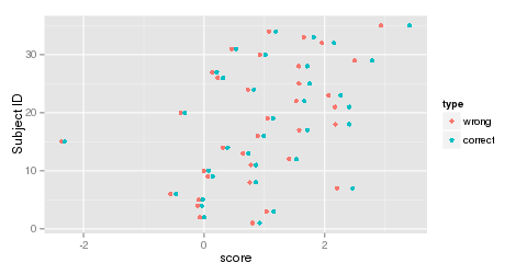
Figure 6: EAP scores with a standard Normal latent distribution (wrong) and estimated Normal distribution (correct).
e1Grp <- list(spec=panas2Grp$spec,
           param=panas2Grp$param,
           data=data)
e1Grp <- panas2Grp
e1Grp$data <- data
s1 <- EAPscores(e1Grp)[,1]  #wrong

e1Grp <- as.IFAgroup(e1Model$panas)
s2 <- EAPscores(e1Grp)[,1]  #correct
It is instructive to see what happens when an e1Grp object is created that omits the estimated latent distribution. Without an explicit latent distribution, the standard Normal is assumed. Examine the change in EAP scores with and without the estimated latent distribution (Figure 6).
Two-Tier Latent Covariance
Suppose a music researcher published item parameters for a measure of music perception accuracy. Items load to some extent on a tonal factor and a rhythm factor. In addition, there are 3 items associated with each stimulus. Since questions asking about the same stimulus are expected to be more correlated than items about different stimulus, these groups of items share extra variance. You have administered this measure to a few classes of music students and wish to know about the distribution of their tonal and rhythmic perception accuracy.
# replace with published item parameters
spec <- list()
spec[1:21] <- rpf.grm(factors=9, outcomes=5)
factors <- c('tonal', 'rhythm', paste('s', 1:7, sep=""))
imat <- mxMatrix(name="item", values=simplify2array(lapply(spec, rpf.rparam)),
              dimnames=list(c(factors, paste('b', 1:4, sep="")),
                            paste("i", 1:length(spec), sep="")))

# arrange the per-stimulus covariance structure
for (stimulus in 1:7) {
  imat$values[2 + stimulus, -(((stimulus - 1) * 3 + 1) : (stimulus*3))] <- 0
}

# replace with your own data
require(MASS)  # for mvrnorm
simCov <- matrix(0, length(factors), length(factors))
diag(simCov) <- rlnorm(length(factors), .5, .5)
simCov[1:2, 1:2] <- c(1.2, .4, .4, .8)
skill <- mvrnorm(200, c(1.1, .7, runif(7)), simCov)
data <- rpf.sample(t(skill), spec, imat$values)

# set up the matrices to hold our latent free parameters
mMat <- mxMatrix(name="mean", nrow=length(factors), ncol=1, values=0, free=TRUE)
rownames(mMat) <- factors
covMat <- mxMatrix(name="cov", values=diag(length(factors)), free=FALSE)
covMat$labels[1,2] <- covMat$labels[2,1] <- 'cov1'  # ensure symmetric
dimnames(covMat) <- list(factors, factors)
covMat$free[1:2, 1:2] <- TRUE
diag(covMat$free) <- TRUE

trModel <- mxModel(model="tr", mMat, covMat, imat,
             mxExpectationBA81(spec, qpoints=15, qwidth=5),
             mxFitFunctionML(),
             mxData(observed=data, type="raw"))

latentModel <- mxModel(model="latent",
                   mxDataDynamic(type="cov", expectation="tr.expectation"),
                   mxExpectationNormal(covariance="tr.cov", means="tr.mean"),
                   mxFitFunctionML())

m1Model <- mxModel(model="music1", trModel, latentModel,
                 mxFitFunctionMultigroup(c("tr.fitfunction", "latent.fitfunction")),
                 mxComputeEM('tr.expectation', 'scores',
                         mxComputeGradientDescent(fitfunction="latent.fitfunction"),
                         tolerance=1))

m1Model <- mxRun(m1Model)
There are 9 factors which usually would entail 9 dimensional integration over the latent density. Such high dimensional integration is either intractable or takes a long time to run. However, this model happens to have a two-tier covariance structure that permits analytic reduction to 3 dimensional integration. Formally, a two-tier covariance matrix is restricted to
where the covariance sub-matrix  is unrestricted (subject to identification),
covariance sub-matrix
is unrestricted (subject to identification),
covariance sub-matrix  is diagonal,
and
is diagonal,
and  is a vector of variances.
The factors that make up
are called primary factors and the factors that comprise
are called specific factors.
Furthermore, each item is permitted to load on at most one specific factor.
is a vector of variances.
The factors that make up
are called primary factors and the factors that comprise
are called specific factors.
Furthermore, each item is permitted to load on at most one specific factor.
mxExpectationBA81(spec, qpoints=15, qwidth=5)
The default quadrature uses 49 points per dimension.
That works out to  points for 3 dimensions.
To speed things up at the cost of some accuracy,
we reduced the equal-interval quadrature to 15 points,
ranging from Z score -5 to 5.
This reduces the number of quadrature points to
points for 3 dimensions.
To speed things up at the cost of some accuracy,
we reduced the equal-interval quadrature to 15 points,
ranging from Z score -5 to 5.
This reduces the number of quadrature points to  .
.
mxComputeEM('tr.expectation', 'scores',
             mxComputeGradientDescent(fitfunction="latent.fitfunction"),
             tolerance=1)
You may have noticed that latent parameter models have used mxComputeGradientDescent instead of mxComputeNewtonRaphson. That is because the analytic derivatives for the multivariate normal required by the Newton-Raphson optimizer had not been coded into OpenMx at the time of writing. At least for item parameters, the availability of two optimizers offers a way to verify that the optimization algorithm is working. You can always replace mxComputeNewtonRaphson by mxComputeGradientDescent. The optimization will take more time, but you can check whether you arrive at the same optimum. The ability to easily swap-out and replace components of a model is invaluable for debugging unexpected behavior. Finally, the option tolerance=1 is there to terminate optimization early. This is meant to be a quick demonstration and requesting higher accuracy slows down estimation substantially.
- multiple group models
- special features to cope with missing data
- automatic-ish item construction (especially for the nominal model)
- simulation studies
Future Extensions
- In addition to mxExpectationNormal, it should be possible to fit the latent distribution to an arbitrary structural model created using RAM or LISREL notation. Currently, the dimensionality of the latent space is limited by the use of quadrature integration. However, the Metropolis-Hastings Robbins-Monro (MH-RM) algorithm can efficiently fit high-dimensional models [Cai2010]. The MH-RM algorithm would make a useful addition to OpenMx.
- The item matrix could be provided as an arbitrary algebra. This would be a generalization of the linear latent trait model.
| [BockAitkin1981] | Bock, R. D. & Aitkin, M. (1981). Marginal maximum likelihood estimation of item parameters: Application of an EM algorithm. Psychometrika, 46, 443–459. |
| [Cai2010] | Cai, L. (2010). High-dimensional exploratory item factor analysis by a Metropolis–Hastings Robbins–Monro algorithm. Psychometrika, 75(1), 33-57. |
| [CaiYangHansen2011] | (1, 2) Cai, L., Yang, J. S., & Hansen, M. (2011). Generalized full-information item bifactor analysis. Psychological Methods, 16(3), 221-248. |
| [Embretson1996] | Embretson, S. E. (1996). The new rules of measurement. Psychological Assessment, 8(4), 341-349. |
| [OrlandoThissen2000] | Orlando, M. and Thissen, D. (2000). Likelihood-Based Item-Fit Indices for Dichotomous Item Response Theory Models. Applied Psychological Measurement, 24(1), 50-64. |
| [WatsonEtal1988] | Watson, D., Clark, L. A., & Tellegen, A. (1988). Development and validation of brief measures of positive and negative affect: The PANAS scales. Journal of Personality and Social Psychology, 54 (6), 1063. |
| [White1994] | Estimation, Inference and Specification Analysis. Cambridge University Press, Cambridge. |
| [Yen1993] | Yen, W. M. (1993). Scaling performance assessments: Strategies for managing local item dependence. Journal of Educational Measurement, 30, 187-213. |