Genetic Epidemiology, Matrix Specification
Mx is probably most popular in the behavior genetics field, as it was conceived with genetic models in mind, which rely heavily on multiple groups. We introduce here an OpenMx script for the basic genetic model in genetic epidemiologic research, the ACE model. This model assumes that the variability in a phenotype, or observed variable, of interest can be explained by differences in genetic and environmental factors, with A representing additive genetic factors, C shared/common environmental factors and E unique/specific environmental factors (see Neale & Cardon 1992, for a detailed treatment). To estimate these three sources of variance, data have to be collected on relatives with different levels of genetic and environmental similarity to provide sufficient information to identify the parameters. One such design is the classical twin study, which compares the similarity of identical (monozygotic, MZ) and fraternal (dizygotic, DZ) twins to infer the role of A, C and E.
The example starts with the ACE model and includes one submodel, the AE model. It is available in the following file:
A parallel version of this example, using path specification of models rather than matrices, can be found here:
ACE Model: a Twin Analysis
Data
Let us assume you have collected data on a large sample of twin pairs for your phenotype of interest. For illustration purposes, we use Australian data on body mass index (BMI) which are saved in a text file ‘myTwinData.txt’. We use R to read the data into a data.frame and to create two subsets of the data for MZ females (mzData) and DZ females (dzData) respectively with the code below.
require(OpenMx)
require(psych)

# Load Data
data(twinData)
describe(twinData, skew=F)

# Select Variables for Analysis
Vars      <- 'bmi'
nv        <- 1       # number of variables
ntv       <- nv*2    # number of total variables
selVars   <- paste(Vars,c(rep(1,nv),rep(2,nv)),sep="")   #c('bmi1','bmi2')

# Select Data for Analysis
mzData    <- subset(twinData, zyg==1, selVars)
dzData    <- subset(twinData, zyg==3, selVars)

# Generate Descriptive Statistics
colMeans(mzData,na.rm=TRUE)
colMeans(dzData,na.rm=TRUE)
cov(mzData,use="complete")
cov(dzData,use="complete")
Model Specification
There are a variety of ways to set up the ACE model. The most commonly used approach in Mx is to specify three matrices for each of the three sources of variance. The matrix a represents the additive genetic path a, the c matrix is used for the shared environmental path c and the matrix e for the unique environmental path e. The expected variances and covariances between member of twin pairs are typically expressed in variance components (or the square of the path coefficients, i.e.  ,
,  and
and  ). These quantities can be calculated using matrix algebra, by multiplying the a matrix by its transpose t(a), and are called A, C and E respectively. Note that the transpose is not strictly needed in the univariate case, but will allow easier transition to the multivariate case.
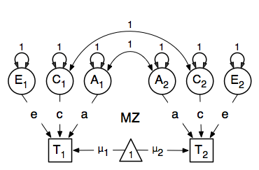
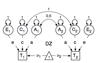
We then use matrix algebra again to add the relevant matrices corresponding to the expectations for each of the statistics of the expected covariance matrix. The R functions cbind and rbind are used to concatenate the resulting matrices in the appropriate way. The expectations can be derived from the path diagrams for MZ and DZ twins. The expectation for the variance of either twin 1 or twin 2 to be included on the diagonal elements is the sum of the variance components (A + C + E). The predicted covariance between MZ twins is a function of their shared genes and environments (A + C). DZ twins on the other hand share only half their genes on average, but the shared environment is by definition also shared completely (.5* A + C).
Note that in R, lower and upper case names are distinguishable so we are using lower case letters for the matrices representing path coefficients a, c and e, rather than X, Y and Z that classic Mx users are familiar with. We continue to use the same upper case letters for matrices representing variance components A, C and E, corresponding to additive genetic (co)variance, shared environmental (co)variance and unique environmental (co)variance respectively, calculated as the square of the path coefficients.
Let’s go through each of the matrices step by step. First, we start with the require(OpenMx) statement. We include the full code here. As MZ and DZ have to be evaluated together, the models for each will be arguments of a bigger model. Given the models for the MZ and the DZ group look rather similar, we start by specifying all the common elements and the model-specific elements which will then be included in the two models (modelMZ and modelDZ) for each of the twin types, defined in separate mxModel commands. The combined model (AceModel) will then include the individual R objects, the MZ and DZ models with their respective R objects as well as the data and a fit function to combine them.
require(OpenMx)

# Set Starting Values
svMe      <- 20      # start value for means
svPa      <- .6      # start value for path coefficients (sqrt(variance/#ofpaths))

# ACE Model
# Matrices declared to store a, d, and e Path Coefficients
pathA     <- mxMatrix( type="Full", nrow=nv, ncol=nv,
                       free=TRUE, values=svPa, label="a11", name="a" )
pathC     <- mxMatrix( type="Full", nrow=nv, ncol=nv,
                       free=TRUE, values=svPa, label="c11", name="c" )
pathE     <- mxMatrix( type="Full", nrow=nv, ncol=nv,
                       free=TRUE, values=svPa, label="e11", name="e" )

# Matrices generated to hold A, C, and E computed Variance Components
covA      <- mxAlgebra( expression=a %*% t(a), name="A" )
covC      <- mxAlgebra( expression=c %*% t(c), name="C" )
covE      <- mxAlgebra( expression=e %*% t(e), name="E" )

# Algebra to compute total variances
covP      <- mxAlgebra( expression=A+C+E, name="V" )

# Algebra for expected Mean and Variance/Covariance Matrices in MZ & DZ twins
meanG     <- mxMatrix( type="Full", nrow=1, ncol=ntv,
                       free=TRUE, values=svMe, label="mean", name="expMean" )
covMZ     <- mxAlgebra( expression=rbind( cbind(V, A+C),
                                          cbind(A+C, V)), name="expCovMZ" )
covDZ     <- mxAlgebra( expression=rbind( cbind(V, 0.5%x%A+ C),
                                          cbind(0.5%x%A+C , V)), name="expCovDZ" )

# Data objects for Multiple Groups
dataMZ    <- mxData( observed=mzData, type="raw" )
dataDZ    <- mxData( observed=dzData, type="raw" )

# Objective objects for Multiple Groups
expMZ     <- mxExpectationNormal( covariance="expCovMZ", means="expMean",
                                  dimnames=selVars )
expDZ     <- mxExpectationNormal( covariance="expCovDZ", means="expMean",
                                  dimnames=selVars )
funML     <- mxFitFunctionML()

# Combine Groups
pars      <- list( pathA, pathC, pathE, covA, covC, covE, covP )
modelMZ   <- mxModel( pars, meanG, covMZ, dataMZ, expMZ, funML, name="MZ" )
modelDZ   <- mxModel( pars, meanG, covDZ, dataDZ, expDZ, funML, name="DZ" )
fitML     <- mxFitFunctionMultigroup(c("MZ.fitfunction","DZ.fitfunction") )
AceModel  <- mxModel( "ACE", pars, modelMZ, modelDZ, fitML )

# Run ADE model
AceFit    <- mxRun(AceModel, intervals=T)
AceSumm   <- summary(AceFit)
AceSumm
Each line can be pasted into R, and then evaluated together once the whole model is specified. First, we create R objects to hold start values for the means (svMe) and the path coefficients (svPA) of the model. For the latter, we use the value of the variance divided by the number of variance components (paths) and take the square root.
# Set Starting Values
svMe      <- 20      # start value for means
svPa      <- .6      # start value for path coefficients (sqrt(variance/#ofpaths))
Given the current example is univariate (in the sense that we analyze one variable, even though we have measured it in two members of twin pairs), the matrices for the paths a, c and e are all Full nv x nv matrices, with nv defined as 1 above, assigned the free status TRUE and given a 0.6 starting value.
# ACE Model
# Matrices declared to store a, d, and e Path Coefficients
pathA     <- mxMatrix( type="Full", nrow=nv, ncol=nv,
                       free=TRUE, values=svPa, label="a11", name="a" )
pathC     <- mxMatrix( type="Full", nrow=nv, ncol=nv,
                       free=TRUE, values=svPa, label="c11", name="c" )
pathE     <- mxMatrix( type="Full", nrow=nv, ncol=nv,
                       free=TRUE, values=svPa, label="e11", name="e" )
While the names of these path coefficient matrices are given lower case names, similar to the convention that paths have lower case names, the names for the variance component matrices, obtained from multiplying matrices with their transpose have upper case letters “A”, “C” and “E” which are distinct (as R is case-sensitive). Note that the label in the matrices above is distinct from the matrix names with 11 referring to the first row and column of the matrix. We also use an mxAlgebra to generate the predicted variance as the sum of the variance components.
# Matrices generated to hold A, C, and E computed Variance Components
covA      <- mxAlgebra( expression=a %*% t(a), name="A" )
covC      <- mxAlgebra( expression=c %*% t(c), name="C" )
covE      <- mxAlgebra( expression=e %*% t(e), name="E" )

# Algebra to compute total variances
covP      <- mxAlgebra( expression=A+C+E, name="V" )
As the focus is on individual differences, the model for the means is typically simple. We can estimate each of the means, in each of the two groups (MZ & DZ) as free parameters. Alternatively, we can establish whether the means can be equated across order and zygosity by fitting submodels to the saturated model. In this case, we opted to use one ‘grand’ mean, obtained by assigning the same label to the elements of the matrix expMean which is a Full 1 x ntv matrix, where ntv is the number of total variables, with free element, labeled mean and given a start value of 20. Note that the R object is called meanG, which becomes an argument of the two respective models. The expMean matrix name defined in the model is then used in both the MZ and DZ model expectations so that all four elements representing means are equated.
# Algebra for expected Mean
meanG     <- mxMatrix( type="Full", nrow=1, ncol=ntv,
                       free=TRUE, values=svMe, label="mean", name="expMean" )
Previous Mx users will likely be familiar with the look of the expected covariance matrices for MZ and DZ twin pairs. These 2x2 matrices are built by horizontal and vertical concatenation of the appropriate matrix expressions for the variance, the MZ or the DZ covariance. In R, concatenation of matrices is accomplished with the rbind and cbind functions. Thus to represent the matrices in expression below in R, we use the following code.
![\begin{eqnarray*}
covMZ = \left[ \begin{array}{c c} a^2+c^2+e^2 & a^2+c^2 \\
a^2+c^2 & a^2+c^2+e^2 \end{array} \right]
\end{eqnarray*}
\begin{eqnarray*}
covDZ = \left[ \begin{array}{c c} a^2+c^2+e^2 & .5a^2+c^2 \\
.5a^2+c^2 & a^2+c^2+e^2 \end{array} \right]
\end{eqnarray*}](_images/math/71a0cac2fc2c919a7530d3ef1bca15c41c655db7.png)
# Algebra for expected and Variance/Covariance Matrices in MZ & DZ twins
covMZ     <- mxAlgebra( expression=rbind( cbind(V, A+C),
                                          cbind(A+C, V)), name="expCovMZ" )
covDZ     <- mxAlgebra( expression=rbind( cbind(V, 0.5%x%A+ C),
                                          cbind(0.5%x%A+ C, V)), name="expCovDZ" )
Next, the observed data are put in a mxData object which also includes a type argument, such that OpenMx can apply the appropriate fit function. The actual model expectations are combined in the mxExpectationNormal statements which reference the respective predicted covariance matrix, predicted means and list of selected variables to map them onto the data. The maximum likelihood fit function mxFitFunction() is used to obtain ML estimates of the parameters of the model.
# Data objects for Multiple Groups
dataMZ    <- mxData( observed=mzData, type="raw" )
dataDZ    <- mxData( observed=dzData, type="raw" )

# Objective objects for Multiple Groups
expMZ     <- mxExpectationNormal( covariance="expCovMZ", means="expMean",
                                  dimnames=selVars )
expDZ     <- mxExpectationNormal( covariance="expCovDZ", means="expMean",
                                  dimnames=selVars )
funML     <- mxFitFunctionML()
As the expected covariance matrices are different for the two groups of twins, we specify two mxModel commands which are given a distinct name and arguments for the predicted means and covariances, the data and the objective function to be used to optimize the model. The objects that are common to both models are combined in a list pars which is then included in both the MZ and DZ models and the overall model, which contains the two other models as arguments, as well as the mxFitFunctionMultigroup to evaluate both models simultaneously. We refer to the correct fit function by adding the name of the model to the two-level argument, i.e. MZ.fitfunction.
# Combine Groups
pars      <- list( pathA, pathC, pathE, covA, covC, covE, covP )
modelMZ   <- mxModel( pars, meanG, covMZ, dataMZ, expMZ, funML, name="MZ" )
modelDZ   <- mxModel( pars, meanG, covDZ, dataDZ, expDZ, funML, name="DZ" )
fitML     <- mxFitFunctionMultigroup(c("MZ.fitfunction","DZ.fitfunction") )
AceModel  <- mxModel( "ACE", pars, modelMZ, modelDZ, fitML )
Model Fitting
We need to invoke the mxRun command to start the model evaluation and optimization. Detailed output will be available in the resulting object, which can be obtained by a summary statement.
# Run ADE model
AceFit    <- mxRun(AceModel, intervals=T)
AceSumm   <- summary(AceFit)
AceSumm
Often, however, one is interested in specific parts of the output. In the case of twin modeling, we typically will inspect the expected covariance matrices and mean vectors, the parameter estimates, and possibly some derived quantities, such as the standardized variance components, obtained by dividing each of the components by the total variance. Note in the code below that the mxEval command allows easy extraction of the values in the various matrices/algebras which form the first argument, with the model name as second argument. Once these values have been put in new objects, we can use and regular R expression to derive further quantities or organize them in a convenient format for including in tables. Note that helper functions could (and will likely) easily be written for standard models to produce ‘standard’ output.
# Generate ACE Model Output
estMean   <- mxEval(expMean, AceFit$MZ)       # expected mean
estCovMZ  <- mxEval(expCovMZ, AceFit$MZ)      # expected covariance matrix for MZ's
estCovDZ  <- mxEval(expCovDZ, AceFit$DZ)      # expected covariance matrix for DZ's
estVA     <- mxEval(a*a, AceFit)              # additive genetic variance, a^2
estVC     <- mxEval(c*c, AceFit)              # dominance variance, d^2
estVE     <- mxEval(e*e, AceFit)              # unique environmental variance, e^2
estVP     <- (estVA+estVC+estVE)              # total variance
estPropVA <- estVA/estVP                      # standardized additive genetic variance
estPropVC <- estVC/estVP                      # standardized dominance variance
estPropVE <- estVE/estVP                      # standardized unique environmental variance
estACE    <- rbind(cbind(estVA,estVC,estVE),  # table of estimates
                   cbind(estPropVA,estPropVC,estPropVE))
LL_ACE    <- mxEval(objective, AceFit)        # likelihood of ADE model
Alternative Models: an AE Model
To evaluate the significance of each of the model parameters, nested submodels are fit in which these parameters are fixed to zero. If the likelihood ratio test between the two models is significant, the parameter that is dropped from the model significantly contributes to the phenotype in question. Here we show how we can fit the AE model as a submodel with a change in one mxMatrix command. First, we call up the previous ‘full’ model as the first argument of a new model AeModel and give it a new name AE. Next we re-specify the matrix c to be fixed to zero by changing the attributes associated with the specific parameter c11 to fixed at zero using a omxSetParameters command. We can run this model in the same way as before and generate similar summaries of the results.
# Run AE model
AeModel   <- mxModel( AceFit, name="AE" )
AeModel   <- omxSetParameters( AeModel, labels="c11", free=FALSE, values=0 )
AeFit     <- mxRun(AeModel)

# Generate AE Model Output
estVA     <- mxEval(a*a, AeFit)               # additive genetic variance, a^2
estVE     <- mxEval(e*e, AeFit)               # unique environmental variance, e^2
estVP     <- (estVA+estVE)                    # total variance
estPropVA <- estVA/estVP                      # standardized additive genetic variance
estPropVE <- estVE/estVP                      # standardized unique environmental variance
estAE     <- rbind(cbind(estVA,estVE),        # table of estimates
                   cbind(estPropVA,estPropVE))
LL_AE     <- mxEval(objective, AeFit)         # likelihood of AE model
We use a likelihood ratio test (or take the difference between -2 times the log-likelihoods of the two models) to determine the best fitting model, and print relevant output.
LRT_ACE_AE <- LL_AE - LL_ACE

#Print relevant output
estACE
estAE
LRT_ACE_AE
These models may also be specified using paths instead of matrices, which allow for easier submodel specification. See Genetic Epidemiology, Path Specification for path specification of these models.