CSOLNP Documentation
CSOLNP is an open-source optimizer engine for the OpenMx package. It is a C++ translation of solnp function from the Rsolnp package, available on CRAN. The algorithm solves nonlinear programming problems in general form of:
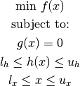
 : Vector of decision variables (
 ).
). : Objective function (
 ).
). : Equality constraint function (
 ).
). : Inequality constraint function (
 ).
). ,
,  : Lower and upper bounds for Inequality constraints.
 ,
,  : Lower and upper bounds for decision variables.
, and are all smooth functions.
Each major iteration of the optimization algorithm solves an augmented Lagrange multiplier method in the form of:
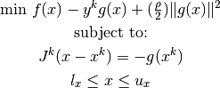
 is the penalty parameter. denotes all the constraints including equality constraints and inequality constraints, which are converted to equalities by adding slack variables.
  is the Jacobian of first derivatives of , and
  is the vector of Lagrange multipliers. The superscript
  denotes the
  major iteration.
Each major iteration starts with a feasibility check of the decision variables  , and continues by implementing a Sequential Quadratic Programming (SQP) method, which calculates the gradient and the Hessian for the augmented Lagrange multiplier method.
The criteria for moving to the next major iteration is satisfied when a Quadratic Programming problem of the form:
, and continues by implementing a Sequential Quadratic Programming (SQP) method, which calculates the gradient and the Hessian for the augmented Lagrange multiplier method.
The criteria for moving to the next major iteration is satisfied when a Quadratic Programming problem of the form:
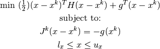
results in a feasible and optimal solution to the augmented Lagrange multiplier problem. If the solution is not feasible or optimal, a new QP problem is called (minor iteration) for updating the gradient and the Hessian. The stop criterion for the optimization is either when the optimal solution is found, or when the maximum number of iterations is reached.
Input
: The penalty parameter in the augmented objective function with the default value of 1. : Step size in numerical gradient calculation with the default value of 1e-7.
Output
Example
To be provided
Restoring NPSOL
To use NPSOL, your OpenMx must be compiled to include it. If NPSOL is available, you can make it the default optimizer with
You can also control this setting with the IMX_OPT_ENGINE environment variable.
Comparing the performances of CSOLNP, and NPSOL
Running the test suite of the package with both optimizers resulted in the following average running times: