Ordinal and Joint Ordinal-Continuous Model Specification
This chapter deals with the specification of models that are either fit exclusively to ordinal variables or to a mix of ordinal and continuous variables. It extends the continuous data common factor model found in previous chapters to ordinal data.
The examples for this chapter can be found in the following files:
The continuous version of this model for raw data can be found the previous demos here:
We will also discuss an example with simulated ordinal data using a regular matrix specification and an alternative one. We will discuss a common factor model with several indicators. This example can be found in the following files:
Ordinal Data Modeling
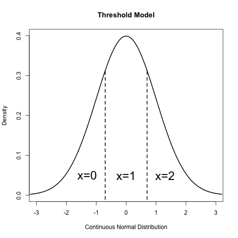
OpenMx models ordinal data under a threshold model. A continuous normal distribution is assumed to underly every ordinal variable. These latent continuous distributions are only observed as being above or below a threshold, where there is one fewer threshold than observed categories in the data. For example, consider a variable with three ordered categories indicated by the values zero, one and two. Under this approach, this variable is assumed to follow a normal distribution that is partitioned or cut by two thresholds: individuals with underlying scores below the first threshold have an observed value of zero, individuals with latent scores between the thresholds are observed with values of one, and individuals with underlying scores give observed values of two.
Each threshold may be freely estimated or assigned as a fixed parameter, depending on the desired model. In addition to the thresholds, ordinal variables still have a mean and variance that describes the parameters of the underlying continuous distribution. However, this underlying distribution must be scaled by fixing at least two parameters to identify the model. One method of identification fixes the mean and variance to specific values, most commonly to a standard normal distribution with a mean of zero and a variance of one. A variation on this method fixes the residual variance of the categorical variable to one, which is often easier to specify. Alternatively, categorical variables may be identified by fixing two thresholds to non-equivalent constant values. These methods will differ in the scale assigned to the ordinal variables (and thus, the scale of the parameters estimated from them), but all identify the same model and should provide equally valid results.
OpenMx allows for the inclusion of continuous and ordinal variables in the same model, as well as models with only continuous or only ordinal variables. Any number of continuous variables may be included in an OpenMx model; however, maximum likelihood estimation for ordinal data must be limited to twenty ordinal variables regardless of the number of continuous variables. Further technical details on ordinal and joint continuous-ordinal optimization are contained at the end of this chapter.
Data Specification
To use ordinal variables in OpenMx, users must identify ordinal variables by specifying those variables as ordered factors in the included data. Ordinal models can only be fit to raw data; if data is described as a covariance or other moment matrix, then the categorical nature of the data was already modeled to generate that moment matrix. Ordinal variables must be defined as specific columns in an R data frame.
Factors are a type of variable included in an R data frame. Unlike numeric or continuous variables, which must include only numeric and missing values, observed values for factors are treated as character strings. All factors contain a levels argument, which lists the possible values for a factor. Ordered factors contain information about the ordering of possible levels. Both R and OpenMx have tools for manipulating factors in data frames. The R functions factor() and as.factor() (and companions ordered() and as.ordered()) can be used to specify ordered factors. OpenMx includes a helper function mxFactor() which more directly prepares ordinal variables as ordered factors in preparation for inclusion in OpenMx models. The code below demonstrates the mxFactor() function, replacing the variable z1 that was initially read as a continuous variable and treating it as an ordinal variable with two levels. This process is repeated for z2 (two levels) and z3 (three levels).
data(myFADataRaw)

oneFactorOrd <- myFADataRaw[,c("z1", "z2", "z3")]

oneFactorOrd$z1 <- mxFactor(oneFactorOrd$z1, levels=c(0, 1))
oneFactorOrd$z2 <- mxFactor(oneFactorOrd$z2, levels=c(0, 1))
oneFactorOrd$z3 <- mxFactor(oneFactorOrd$z3, levels=c(0, 1, 2))
Threshold Specification
Just as covariances and means are included in models by specifying matrices and algebras, thresholds may be included in models as threshold matrices. These matrices can be of user-specified type, though most will be of type Full. The columns of this matrix should correspond to the ordinal variables in your dataset, with the column names of this matrix corresponding to variables in your data. This assignment can be done either with the dimnames argument to mxMatrix, or by using the threshnames argument in your expectation function the same way dimnames arguments are used. The rows of your threshold matrix should correspond to the ordered thresholds for each variable, such that the first row is the lowest threshold for each variable, the second row is the next threshold (provided one or more of your variables have two thresholds), and so on for the maximum number of thresholds you have in your data. Rows of the threshold matrix beyond the number of thresholds in a particular variable should be fixed parameters with starting values of NA.
As an example, the data prep example above includes two binary variables (z1 and z2) and one variable with three categories (z3). This means that the threshold matrix for models fit to this data should contain three columns (for z1, z2 and z3) and two rows, as the variable z3 requires two thresholds. The code below specifies a 2 x 3 Full matrix with free parameters for one threshold for z1, one threshold for z2 and two thresholds for z3.
thresh       <- mxMatrix( type="Full", nrow=2, ncol=3,
                          free=c(TRUE,TRUE,TRUE,FALSE,FALSE,TRUE),
                          values=c(-1,0,-.5,NA,NA,1.2), byrow=TRUE, name="thresh" )
There are a few common errors regarding the use of thresholds in OpenMx. First, threshold values within each row must be strictly increasing, such that the value in any element of the threshold matrix must be greater than all values above it in that column. In the above example, the second threshold for z3 is set at 1.2, above the value of -.5 for the first threshold. OpenMx will return an error when your thresholds are not strictly increasing. There are no restrictions on values across columns or variables: the second threshold for z3 could be below all thresholds for z1 and z2 provided it exceeded the value for the first z3 threshold. Second, the dimnames of the threshold matrix must match ordinal factors in the data. Additionally, free parameters should only be included for thresholds present in your data: including a second freely estimated threshold for z1 or z2 in this example would not directly impede model estimation, but would remain at its starting value and count as a free parameter for the purposes of calculating fit statistics.
It is also important to remember that specifying a threshold matrix is not sufficient to get an ordinal data model to run. In addition, the scale of each ordinal variable must be identified just like the scale of a latent variable. The most common method for this involves constraining a ordinal item’s mean to zero and either its total or residual variance to a constant value (i.e., one). For variables with two or more thresholds, ordinal variables may also be identified by constraining two thresholds to fixed values. Models that don’t identify the scale of their ordinal variables should not converge.
While thresholds can’t be expressed as paths between variables like other parts of the model, OpenMx supports a path-like interface called mxThreshold as of version 2.0. This function is described in more detail in the ordinal data version of this chapter and the mxThreshold help file.
Users of original or ‘’classic’’ Mx may recall specifying thresholds not in absolute terms, but as deviations. This method estimated the difference between each threshold for a variable and the previous one, which ensured that thresholds were in the correct order (i.e., that the second threshold for a variable was not lower than the first). While users may employ this method using mxAlgebra as it suits them, OpenMx does not require this technique. Simply specifying a thresholds matrix is typically sufficient to keep thresholds in proper order.
Including Thresholds in Models
Finally, the threshold matrix must be identified as such in the expectation function in the same way that other matrices are identified as means or covariance matrices. Both the mxExpectationNormal and mxExpectationRAM contain a thresholds argument, which takes the name of the matrix or algebra to be used as the threshold matrix for a given analysis. Although specifying type='RAM' generates a RAM expectation function, this expectation function must be replaced by one with a specified thresholds matrix.
You must specify dimnames (dimension names) for your thresholds matrix that correspond to the ordered factors in the data you wish to analyze. This may be done in either of two ways, both of which correspond to specifying dimnames for other OpenMx matrices. One method is to use the threshnames argument in the mxExpectationNormal or mxExpectationRAM functions, which specifies which variables are in a threshold matrix in the same way the dimnames argument specifies which variables are in the rest of the model. Another method is to specify dimnames for each matrix using the dimnames argument in the mxMatrix function. Either method may be used, but it is important to use the same method for all matrices in a given model (either using expectation function arguments dimnames and threshnames or supplying dimnames for all mxMatrix objects manually). Expectation function arguments dimnames and threshnames supersede the matrix dimname arguments, and threshnames will take the value of the dimnames if both dimnames and thresholds are specified but threshnames is omitted.
The code below specifies an mxExpectationRAM to include a thresholds matrix named "thresh". When models are built using type='RAM', the dimnames argument may be omitted, as the requisite dimnames for the A, S, F and M matrices are generated from the manifestVars and latentVars lists. However, the dimnames for the threshold matrix should be included using the dimnames argument in mxMatrix.
mxExpectationRAM(A="A", S="S", F="F", M="M", thresholds="thresh")
Common Factor Model
All of the raw data examples through the documentation may be converted to ordinal examples by the inclusion of ordinal data, the specification of a threshold matrix and inclusion of that threshold matrix in the objective function.
Ordinal Data
The following example is a version of the continuous data common factor model referenced at the beginning of this chapter. Aside from replacing the continuous variables x1-x6 with the ordinal variables z1-z3, the code below simply incorporates the steps referenced above into the existing example. Data preparation occurs first, with the added mxFactor statements to identify ordinal variables and their ordered levels.
require(OpenMx)

data(myFADataRaw)

oneFactorOrd <- myFADataRaw[,c("z1", "z2", "z3")]

oneFactorOrd$z1 <- mxFactor(oneFactorOrd$z1, levels=c(0, 1))
oneFactorOrd$z2 <- mxFactor(oneFactorOrd$z2, levels=c(0, 1))
oneFactorOrd$z3 <- mxFactor(oneFactorOrd$z3, levels=c(0, 1, 2))
Model specification can be achieved by appending the above threshold matrix and expectation function to either the path or matrix common factor examples. The path example below has been altered by changing the variable names from x1-x6 to z1-z3, adding the threshold matrix and expectation function, and identifying the ordinal variables by constraining their means to be zero and their residual variances to be one.
dataRaw      <- mxData(oneFactorOrd, type="raw")
# asymmetric paths
matrA        <- mxMatrix( type="Full", nrow=4, ncol=4,
                          free=c(F,F,F,T,
                                 F,F,F,T,
                                 F,F,F,T,
                                 F,F,F,F),
                          values=c(0,0,0,1,
                                   0,0,0,1,
                                   0,0,0,1,
                                   0,0,0,0),
                          labels=c(NA,NA,NA,"l1",
                                   NA,NA,NA,"l2",
                                   NA,NA,NA,"l3",
                                   NA,NA,NA,NA),
                          byrow=TRUE, name="A" )
# symmetric paths
matrS        <- mxMatrix( type="Symm", nrow=4, ncol=4,
                          free=FALSE,
                          values=diag(4),
                          labels=c("e1", NA, NA,  NA,
                                    NA,"e2", NA,  NA,
                                    NA,  NA,"e3", NA,
                                    NA,  NA, NA, "varF1"),
                          byrow=TRUE, name="S" )
# filter matrix
matrF        <- mxMatrix( type="Full", nrow=3, ncol=4,
                          free=FALSE, values=c(1,0,0,0,  0,1,0,0,  0,0,1,0),
                          byrow=TRUE, name="F" )
# means
matrM        <- mxMatrix( type="Full", nrow=1, ncol=4,
                          free=FALSE, values=0,
                          labels=c("meanz1","meanz2","meanz3",NA), name="M" )
thresh       <- mxMatrix( type="Full", nrow=2, ncol=3,
                          free=c(TRUE,TRUE,TRUE,FALSE,FALSE,TRUE),
                          values=c(-1,0,-.5,NA,NA,1.2), byrow=TRUE, name="thresh" )
exp          <- mxExpectationRAM("A","S","F","M", dimnames=c("z1","z2","z3","F1"),
                          thresholds="thresh", threshnames=c("z1","z2","z3"))
funML        <- mxFitFunctionML()

oneFactorOrdinalModel <- mxModel("Common Factor Model Matrix Specification",
                                 dataRaw, matrA, matrS, matrF, matrM, thresh, exp, funML)
This model may then be optimized using the mxRun command.
oneFactorOrdinalFit <- mxRun(oneFactorOrdinalModel)
Joint Ordinal-Continuous Data
Models with both continuous and ordinal variables may be specified just like any other ordinal data model. Threshold matrices in these models should contain columns only for the ordinal variables, and should contain column names to designate which variables are to be treated as ordinal. In the example below, the one factor model above is estimated with three continuous variables (x1-x3) and three ordinal variables (z1-z3).
require(OpenMx)

oneFactorJoint <- myFADataRaw[,c("x1", "x2", "x3", "z1", "z2", "z3")]

oneFactorJoint$z1 <- mxFactor(oneFactorOrd$z1, levels=c(0, 1))
oneFactorJoint$z2 <- mxFactor(oneFactorOrd$z2, levels=c(0, 1))
oneFactorJoint$z3 <- mxFactor(oneFactorOrd$z3, levels=c(0, 1, 2))

dataRaw      <- mxData(observed=oneFactorJoint, type="raw")
# asymmetric paths
matrA        <- mxMatrix( type="Full", nrow=7, ncol=7,
                          free=c(rep(c(F,F,F,F,F,F,T),6),rep(F,7)),
                          values=c(rep(c(0,0,0,0,0,0,1),6),rep(F,7)),
                          labels=rbind(cbind(matrix(NA,6,6),matrix(paste("l",1:6,sep=""),6,1)),
                           matrix(NA,1,7)),
                          byrow=TRUE, name="A" )
# symmetric paths
labelsS      <- matrix(NA,7,7); diag(labelsS) <- c(paste("e",1:6,sep=""),"varF1")
matrS        <- mxMatrix( type="Symm", nrow=7, ncol=7,
                          free= rbind(cbind(matrix(as.logical(diag(3)),3,3),matrix(F,3,4)),
                           matrix(F,4,7)),
                          values=diag(7), labels=labelsS, byrow=TRUE, name="S" )
# filter matrix
matrF        <- mxMatrix( type="Full", nrow=6, ncol=7,
                          free=FALSE, values=cbind(diag(6),matrix(0,6,1)),
                          byrow=TRUE, name="F" )
# means
matrM        <- mxMatrix( type="Full", nrow=1, ncol=7,
                          free=c(T,T,T,F,F,F,F), values=c(1,1,1,0,0,0,0),
                          labels=c("meanx1","meanx2","meanx3","meanz1","meanz2","meanz3",NA),
                          name="M" )
thresh       <- mxMatrix( type="Full", nrow=2, ncol=3,
                          free=c(TRUE,TRUE,TRUE,FALSE,FALSE,TRUE),
                          values=c(-1,0,-.5,NA,NA,1.2), byrow=TRUE, name="thresh" )
exp          <- mxExpectationRAM("A","S","F","M",
                                 dimnames=c("x1","x2","x3","z1","z2","z3","F1"),
                                 thresholds="thresh", threshnames=c("z1","z2","z3"))
funML        <- mxFitFunctionML()

oneFactorJointModel <- mxModel("Common Factor Model Matrix Specification",
                               dataRaw, matrA, matrS, matrF, matrM, thresh, exp, funML)
This model may then be optimized using the mxRun command.
oneFactorJointFit <- mxRun(oneFactorJointModel)
Simulated Ordinal Data
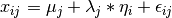
The common factor model is a method for modeling the relationships between observed variables believed to measure or indicate the same latent variable. While there are a number of exploratory approaches to extracting latent factor(s), this example uses structural modeling to fit a confirmatory factor model. The model for any person and path diagram of the common factor model for a set of variables  -
-  are given below.
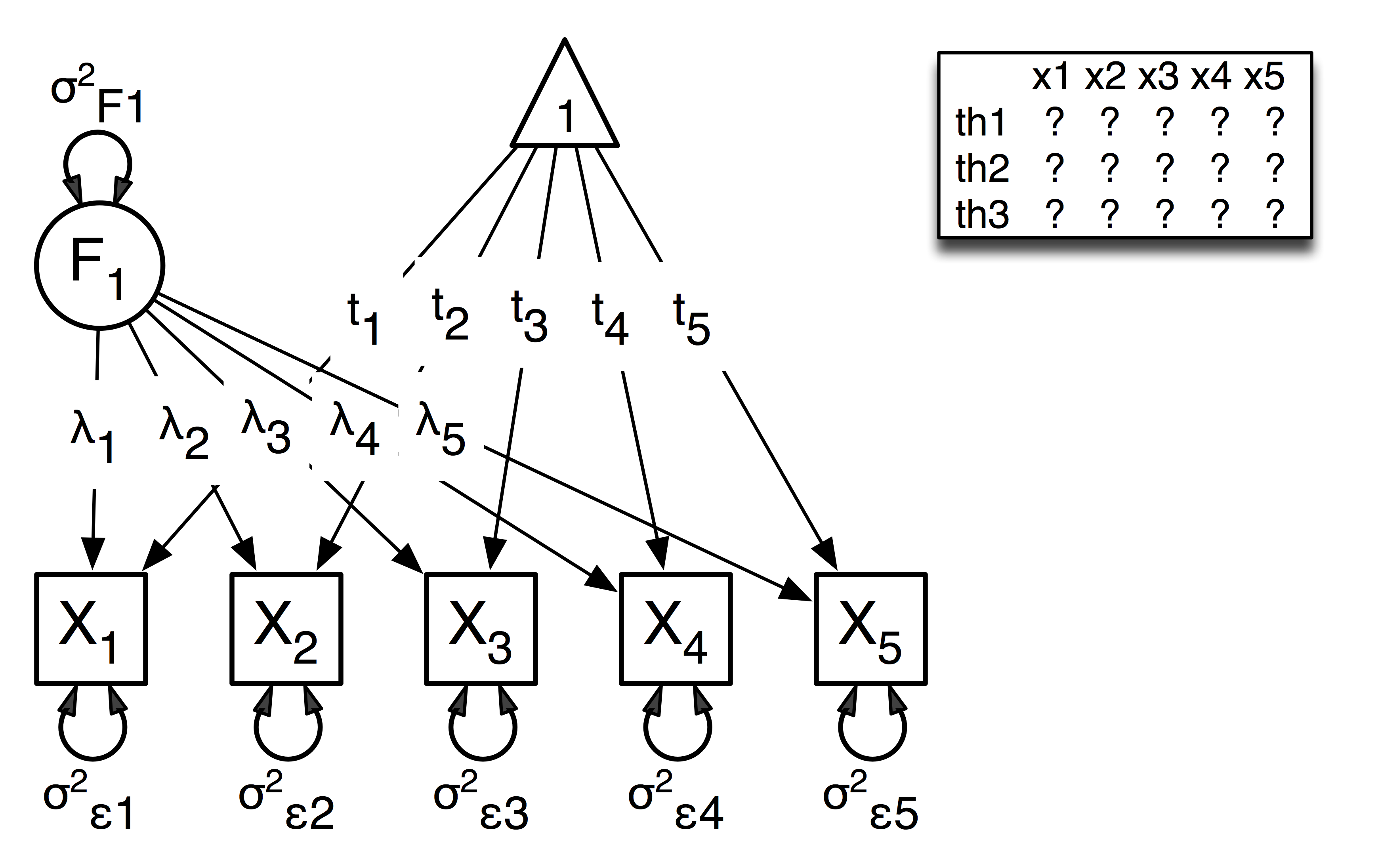
The path diagram above displays 16 parameters (represented in the arrows: 5 manifest variances, five manifest means, five factor loadings and one factor variance). However, given we are dealing with ordinal data in this example, we are estimating thresholds rather than means, with nThresholds being one less the number of categories in the variables, here 3. Furthermore, we must constrain either the factor variance or one factor loading to a constant to identify the model and scale the latent variable. In this instance, we chose to constrain the variance of the factor. We also need to constrain the total variances of the manifest variables, as ordinal variables do not have a scale of measurement. As such, this model contains 20 free parameters and is not fully saturated.
Data
Our first step to running this model is to include the data to be analyzed. The data for this example were simulated in R. Given the focus of this documentation is on OpenMx, we will not discuss the details of the simulation here, but we do provide the code so that the user can simulate data in a similar way.
# Step 1: set up simulation parameters
# Note: nVariables>=5, nThresholds>=1, nSubjects>=nVariables x nThresholds
# (maybe more) and model should be identified
nVariables   <-5
nFactors     <-1
nThresholds  <-3
nSubjects    <-500
isIdentified <- function(nVariables,nFactors)
    as.logical(1+sign((nVariables*(nVariables-1)/2)
    - nVariables*nFactors + nFactors*(nFactors-1)/2))
# if this function returns FALSE then model is not identified, otherwise it is.
isIdentified(nVariables,nFactors)

loadings     <- matrix(.7,nrow=nVariables,ncol=nFactors)
residuals    <- 1-(loadings * loadings)
sigma        <- loadings %*% t(loadings) + vec2diag(residuals)
mu           <- matrix(0,nrow=nVariables,ncol=1)

# Step 2: simulate multivariate normal data
set.seed(1234)
continuousData <- mvrnorm(n=nSubjects,mu,sigma)

# Step 3: chop continuous variables into ordinal data
# with nThresholds+1 approximately equal categories, based on 1st variable
quants       <- quantile(continuousData[,1],  probs = c((1:nThresholds)/(nThresholds+1)))
ordinalData  <- matrix(0,nrow=nSubjects,ncol=nVariables)
for(i in 1:nVariables)
{ ordinalData[,i] <- cut(as.vector(continuousData[,i]),c(-Inf,quants,Inf)) }

# Step 4: make the ordinal variables into R factors
ordinalData  <- mxFactor(as.data.frame(ordinalData),levels=c(1:(nThresholds+1)))

# Step 5: name the variables
bananaNames  <- paste("banana",1:nVariables,sep="")
names(ordinalData) <- bananaNames
Model Specification
The following code contains all of the components of our model. Before running a model, the OpenMx library must be loaded into R using either the require() or library() function. All objects required for estimation (data, matrices, an expectation function, and a fit function) are included in their functions. This code uses the mxModel function to create an MxModel object, which we will then run. We pre-specify a number of ‘variables’, namely the number of variables analyzed nVariables, in this case 5, the number of factors nFactors, here one, and the number of thresholds nThresholds, here 3 or one less than the number of categories in the simulated ordinal variable.
facLoads     <- mxMatrix( type="Full", nrow=nVariables, ncol=nFactors,
                          free=TRUE, values=0.2, lbound=-.99, ubound=.99, name="facLoadings" )
vecOnes      <- mxMatrix( type="Unit", nrow=nVariables, ncol=1, name="vectorofOnes" )
resVars      <- mxAlgebra( expression=vectorofOnes -
                           (diag2vec(facLoadings %*% t(facLoadings))), name="resVariances" )
expCovs      <- mxAlgebra( expression=facLoadings %*% t(facLoadings)
                           + vec2diag(resVariances), name="expCovariances" )
expMeans     <- mxMatrix( type="Zero", nrow=1, ncol=nVariables, name="expMeans" )
threDevs     <- mxMatrix( type="Full", nrow=nThresholds, ncol=nVariables,
                          free=TRUE, values=.2,
                          lbound=rep( c(-Inf,rep(.01,(nThresholds-1))) , nVariables),
                          dimnames=list(c(), bananaNames), name="thresholdDeviations" )
unitLower    <- mxMatrix( type="Lower", nrow=nThresholds, ncol=nThresholds,
                          free=FALSE, values=1, name="unitLower" )
expThres     <- mxAlgebra( expression=unitLower %*% thresholdDeviations,
                           name="expThresholds" )
dataRaw      <- mxData( observed=ordinalData, type='raw' )
exp          <- mxExpectationNormal( covariance="expCovariances", means="expMeans",
                                     dimnames=bananaNames, thresholds="expThresholds" )
funML        <- mxFitFunctionML()

oneFactorThresholdModel <- mxModel("oneFactorThresholdModel", dataRaw,
                                   facLoads, vecOnes, resVars, expCovs, expMeans, threDevs,
                                   unitLower, expThres, dataRaw, exp, funML )
This mxModel function can be split into several parts. First, we give the model a name “Common Factor ThresholdModel Matrix Specification”.
The second component of our code creates an MxData object. The example above, reproduced here, first references the object where our data is, then uses the type argument to specify that this is raw data.
dataRaw <- mxData( observed=ordinalData, type='raw' )
The first mxMatrix statement declares a Full nVariables x nFactors matrix of factor loadings to be estimated, called “facLoadings”, where the rows represent the dependent variables and the column(s) represent the independent variable(s). The common factor model requires that one parameter (typically either a factor loading or factor variance) be constrained to a constant value. In our model, we will constrain the factor variance to 1 for identification, and let all the factor loadings be freely estimated. Even though we specify just one start value of 0.2, it is recycled for each of the elements in the matrix. Given the factor variance is fixed to one, and the variances of the observed variables are fixed to one (see below), the factor loadings are standarized, and thus must lie between -.99 and .99 as indicated by the lbound and ubound values.
# factor loadings
facLoads     <- mxMatrix( type="Full", nrow=nVariables, ncol=nFactors,
                          free=TRUE, values=0.2, lbound=-.99, ubound=.99, name="facLoadings" )
Note that if nFactors>1, we could add a standardized mxMatrix to estimate the correlation between the factors. Such a matrix automatically has 1’s on the diagonal, fixing the factor variances to one and thus allowing all the factor loadings to be estimated. In the current example, all the factor loadings are estimated which implies that the factor variance is fixed to 1. Alternatively, we could add a symmetric 1x1 matrix to estimates the variance of the factor, when one of the factor loadings is fixed.
As our data are ordinal, we further need to constrain the variances of the observed variables to unity. These variances are made up of the contributions of the latent common factor and the residual variances. The amount of variance explained by the common factor is obtained by squaring the factor loadings. We subtract the squared factor loadings from 1 to get the amount explained by the residual variance, thereby implicitly fixing the variances of the observed variables to 1. To do this for all variables simultaneously, we use matrix algebra functions. We first specify a vector of One’s by declaring a Unit nVariables x 1 matrix called vectorofOnes. We need to subtract the squared factor loadings which are on the diagonal of the matrix multiplication of the factor loading matrix facLoadings and its transpose. To extract those into squared factor loadings into a vector, we use the diag2vec function. This new vector is subtracted from the vectorofOnes using an mxAlgebra statement to generate the residual variances, and named resVariances.
vecOnes      <- mxMatrix( type="Unit", nrow=nVariables, ncol=1, name="vectorofOnes" )
# residuals
resVars      <- mxAlgebra( expression=vectorofOnes -
                          (diag2vec(facLoadings %*% t(facLoadings))), name="resVariances" )
We then use the reverse function vec2diag to put the residual variances on the diagonal and add the contributions through the common factor from the matrix multipication of the factor loadings matrix and its transpose to obtain the formula for the expected covariances, aptly named expCovariances.
# expected covariances
expCovs      <- mxAlgebra( expression=facLoadings %*% t(facLoadings)
                           + vec2diag(resVariances), name="expCovariances" )
When fitting to ordinal rather than continuous data, we estimate thresholds rather than means. The matrix of thresholds is of size nThresholds x nVariables where nThresholds is one less than the number of categories for the ordinal variable(s). We still specify a matrix of means, however, it is fixed to zero. An alternative approach is to fix the first two thresholds (to zero and one, see below), which allows us to estimate means and variances in a similar way to fitting to continuous data. Let’s first specify the model with zero means and free thresholds.
The means are specified as a Zero 1 x nVariables matrix, called expMeans. A means matrix always contains a single row, and one column for every manifest variable in the model.
# expected means
expMeans     <- mxMatrix( type="Zero", nrow=1, ncol=nVariables, name="expMeans" )
The mean of the factor(s) is also fixed to 0, which is implied by not including a matrix for it. Alternatively, we could explicitly add a Full 1 x nFactors matrix with a fixed value of zero for the factor mean(s), named “facMeans”.
We estimate the Full nThresholds x nVariables matrix. To make sure that the thresholds systematically increase from the lowest to the highest, we estimate the first threshold and the increments compared to the previous threshold by constraining the increments to be positive. This is accomplished through some R algebra, concatenating minus infinity and (nThreshold-1) times .01 as the lower bound for the remaining estimates. This matrix of thresholdDeviations is then pre-multiplied by a lower triangular matrix of ones of size nThresholds x nThresholds to obtain the expected thresholds in increasing order in the thresholdMatrix.
threDevs     <- mxMatrix( type="Full", nrow=nThresholds, ncol=nVariables,
                          free=TRUE, values=.2,
                          lbound=rep( c(-Inf,rep(.01,(nThresholds-1))) , nVariables),
                          dimnames=list(c(), bananaNames), name="thresholdDeviations" )
unitLower    <- mxMatrix( type="Lower", nrow=nThresholds, ncol=nThresholds,
                          free=FALSE, values=1, name="unitLower" )
# expected thresholds
expThres     <- mxAlgebra( expression=unitLower %*% thresholdDeviations,
                          name="expThresholds" )
The final parts of this model are the expectation function and the fit function. The choice of expectation function determines the required arguments. Here we fit to raw ordinal data, thus we specify the matrices for the expected covariance matrix of the data, as well as the expected means and thresholds previously specified. We use dimnames to map the model for means, thresholds and covariances onto the observed variables.
exp          <- mxExpectationNormal( covariance="expCovariances", means="expMeans",
                                     dimnames=bananaNames, thresholds="expThresholds" )
funML        <- mxFitFunctionML()
The free parameters in the model can then be estimated using full information maximum likelihood (FIML) for covariances, means and thresholds. FIML is specified by using raw data with the mxFitFunctionML. To estimate free parameters, the model is run using the mxRun function, and the output of the model can be accessed from the $output slot of the resulting model. A summary of the output can be reached using summary().
oneFactorThresholdFit <- mxRun(oneFactorThresholdModel)

oneFactorThresholdFit$output
summary(oneFactorThresholdFit)
Alternative Specification
As indicate above, the model can be re-parameterized such that means and variances of the observed variables are estimated similar to the continuous case, by fixing the first two thresholds. This basically rescales the parameters of the model. Below is the full script:
facLoads     <- mxMatrix( type="Full", nrow=nVariables, ncol=nFactors,
                          free=TRUE, values=0.2, lbound=-.99, ubound=2, name="facLoadings" )
resVars      <- mxMatrix( type="Diag", nrow=nVariables, ncol=nVariables,
                          free=TRUE, values=0.9, name="resVariances" )
expCovs      <- mxAlgebra( expression=facLoadings %*% t(facLoadings) + resVariances,
                           name="expCovariances" )
expMeans     <- mxMatrix( type="Full", nrow=1, ncol=nVariables, free=TRUE, name="expMeans" )
threDevs     <- mxMatrix( type="Full", nrow=nThresholds, ncol=nVariables,
                          free=rep( c(F,F,rep(T,(nThresholds-2))), nVariables),
                          values=rep( c(0,1,rep(.2,(nThresholds-2))), nVariables),
                          lbound=rep( c(-Inf,rep(.01,(nThresholds-1))), nVariables),
                          dimnames=list(c(), bananaNames), name="thresholdDeviations" )
unitLower    <- mxMatrix( type="Lower", nrow=nThresholds, ncol=nThresholds,
                          free=FALSE, values=1, name="unitLower" )
expThres     <- mxAlgebra( expression=unitLower %*% thresholdDeviations,
                           name="expThresholds" )

colOnes      <- mxMatrix( type="Unit", nrow=nThresholds, ncol=1, name="columnofOnes" )
matMeans     <- mxAlgebra( expression=expMeans %x% columnofOnes, name="meansMatrix" )
matVars      <- mxAlgebra( expression=sqrt(t(diag2vec(expCovariances))) %x% columnofOnes,
                           name="variancesMatrix" )
matThres     <- mxAlgebra( expression=(expThresholds - meansMatrix) / variancesMatrix,
                           name="thresholdMatrix" )
identity     <- mxMatrix( type="Iden", nrow=nVariables, ncol=nVariables, name="Identity" )
stFacLoads   <- mxAlgebra( expression=solve(sqrt(Identity * expCovariances)) %*% facLoadings,
                           name="standFacLoadings" )
dataRaw      <- mxData( observed=ordinalData, type='raw' )
exp          <- mxExpectationNormal( covariance="expCovariances", means="expMeans",
                                     dimnames=bananaNames, thresholds="expThresholds" )
funML        <- mxFitFunctionML()

oneFactorThreshold01Model <- mxModel("oneFactorThreshold01Model", dataRaw,
                                   facLoads, resVars, expCovs, expMeans, threDevs,
                                   unitLower, expThres,
                                   colOnes, matMeans, matVars, matThres, identity,
                                   stFacLoads, dataRaw, exp, funML )
We will only highlight the changes from the previous model specification. By fixing the first and second threshold to 0 and 1 respectively for each variable, we are now able to estimate a mean and a variance for each variable instead. If we are estimating the variances of the observed variables, the factor loadings are no longer standardized, thus we relax the upper boundary on the factor loading matrix facLoadings to be 2. The residual variances are now directly estimated as a Diagonal matrix of size nVariables x nVariables, and given a start value higher than that for the factor loadings. As the residual variances are already on the diagonal of the resVariances matrix, we no longer need to add the vec2diag function to obtain the expCovariances matrix.
facLoads     <- mxMatrix( type="Full", nrow=nVariables, ncol=nFactors,
                          free=TRUE, values=0.2, lbound=-.99, ubound=2, name="facLoadings" )
resVars      <- mxMatrix( type="Diag", nrow=nVariables, ncol=nVariables,
                          free=TRUE, values=0.9, name="resVariances" )
expCovs      <- mxAlgebra( expression=facLoadings %*% t(facLoadings) + resVariances,
                           name="expCovariances" )
Next, we now estimate the means for the observed variables and thus change the expMeans matrix to a Full matrix, and set it free. The most complicated change happens to the matrix of thresholdDeviations. Its type and dimensions stay the same. However, we now fix the first two thresholds, but allow the remainder of the thresholds (in this case, just one) to be estimated. We use the R rep function to make this happen. The values statement now has the fixed value of 0 for the first threshold, the fixed value of 1 for the second threshold, and the start value of .2 for the remaining threshold(s). Finally, no change is required for the lbound matrix, which is still necessary to keep the estimated increments (third threshold and possible more) positive.
expMeans     <- mxMatrix( type="Full", nrow=1, ncol=nVariables, free=TRUE, name="expMeans" )
threDevs     <- mxMatrix( type="Full", nrow=nThresholds, ncol=nVariables,
                          free=rep( c(F,F,rep(T,(nThresholds-2))), nVariables),
                          values=rep( c(0,1,rep(.2,(nThresholds-2))), nVariables),
                          lbound=rep( c(-Inf,rep(.01,(nThresholds-1))), nVariables),
                          dimnames=list(c(), bananaNames), name="thresholdDeviations" )
These are all the changes required to fit the alternative specification, which should give the same likelihood and goodness-of-fit statistics as the original one. We have added some matrices and algebra to calculate the ‘standardized’ thresholds and factor loadings which should be equal to those obtained with the original specification. To standardize the thresholds, the respective mean is subtracted from the thresholds, by expanding the means matrix to the same size as the threshold matrix. The result is divided by the corresponding standard deviation. To standardize the factor loadings, they are pre-multiplied by the inverse of the standard deviations.
colOnes      <- mxMatrix( type="Unit", nrow=nThresholds, ncol=1, name="columnofOnes" )
matMeans     <- mxAlgebra( expression=expMeans %x% columnofOnes, name="meansMatrix" )
matVars      <- mxAlgebra( expression=sqrt(t(diag2vec(expCovariances))) %x% columnofOnes,
                           name="variancesMatrix" )
matThres     <- mxAlgebra( expression=(expThresholds - meansMatrix) / variancesMatrix,
                           name="thresholdMatrix" )
identity     <- mxMatrix( type="Iden", nrow=nVariables, ncol=nVariables, name="Identity" )
stFacLoads   <- mxAlgebra( expression=solve(sqrt(Identity * expCovariances))
                           %*% facLoadings, name="standFacLoadings" )
Technical Details
Maximum likelihood estimation for ordinal variables by generating expected covariance and mean matrices for the latent continuous variables underlying the set of ordinal variables, then integrating the multivariate normal distribution defined by those covariances and means. The likelihood for each row of the data is defined as the multivariate integral of the expected distribution over the interval defined by the thresholds bordering that row’s data. OpenMx uses Alan Genz’s SADMVN routine for multivariate normal integration (see http://www.math.wsu.edu/faculty/genz/software/software.html for more information).
When continuous variables are present, OpenMx utilizes a block decomposition to separate the continuous and ordinal covariance matrices for FIML. The likelihood of the continuous variables is calculated normally. The effects of the point estimates of the continuous variables is projected out of the expected covariance matrix of the ordinal data. The likelihood of the ordinal data is defined as the multivariate integral over the distribution defined by the resulting ordinal covariance matrix.