Multiple Groups, Matrix Specification
An important aspect of structural equation modeling is the use of multiple groups to compare means and covariances structures between any two (or more) data groups, for example males and females, different ethnic groups, ages etc. Other examples include groups which have different expected covariances matrices as a function of parameters in the model, and need to be evaluated together for the parameters to be identified.
The example includes the heterogeneity model as well as its submodel, the homogeneity model and is available in the following file:
A parallel version of this example, using paths specification of models rather than matrices, can be found here:
Heterogeneity Model
We will start with a basic example here, building on modeling means and variances in a saturated model. Assume we have two groups and we want to test whether they have the same mean and covariance structure.
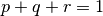
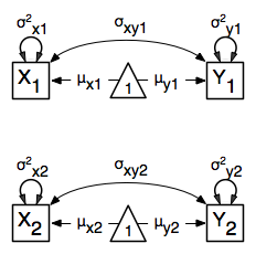
The path diagram of the heterogeneity model for a set of variables  and
and  are given below.
Data
For this example we simulated two datasets (xy1 and xy2) each with zero means and unit variances, one with a correlation of 0.5, and the other with a correlation of 0.4 with 1000 subjects each. We use the mvrnorm function in the MASS package, which takes three arguments: Sample Size, Means, Covariance Matrix). We check the means and covariance matrix in R and provide dimnames for the dataframe. See attached R code for simulation and data summary.
#Simulate Data
require(MASS)
#group 1
set.seed(200)
xy1 <- mvrnorm (1000, c(0,0), matrix(c(1,.5,.5,1),2,2))
#group 2
set.seed(200)
xy2 <- mvrnorm (1000, c(0,0), matrix(c(1,.4,.4,1),2,2))

#Print Descriptive Statistics
selVars <- c('X','Y')
summary(xy1)
cov(xy1)
dimnames(xy1) <- list(NULL, selVars)
summary(xy2)
cov(xy2)
dimnames(xy2) <- list(NULL, selVars)
Model Specification
As before, we include the OpenMx package using a require statement. We first fit a heterogeneity model, allowing differences in both the mean and covariance structure of the two groups. As we are interested whether the two structures can be equated, we have to specify the models for the two groups, named group1 and group2 within another model. The structure of the job thus look as follows, with two mxModel commands as arguments of another mxModel command. Note that mxModel commands are unlimited in the number of arguments.
For each of the groups, we fit a saturated model, using a Cholesky decomposition to generate the expected covariance matrix and a row vector for the expected means. Note that we have specified different labels for all the free elements, in the two mxModel statements. For more details, see example 1.
require(OpenMx)

#Fit Heterogeneity Model

chol1        <- mxMatrix( type="Lower", nrow=2,  ncol=2,
                          free=T, values=.5, labels=c("Ch11","Ch21","Ch31"), name="chol1" )
expCov1      <- mxAlgebra( expression=chol1 %*% t(chol1), name="expCov1" )
expMean1     <- mxMatrix( type="Full", nrow=1, ncol=2,
                          free=T, values=c(0,0), labels=c("mX1","mY1"), name="expMean1" )
dataRaw1     <- mxData( xy1, type="raw" )
exp1         <- mxExpectationNormal( covariance="expCov1", means="expMean1", selVars)
funML        <- mxFitFunctionML()
model1       <- mxModel("group1",
                         dataRaw1, chol1, expCov1, expMean1, exp1, funML)

chol2        <- mxMatrix( type="Lower", nrow=2,  ncol=2,
                          free=T, values=.5, labels=c("Ch12","Ch22","Ch32"), name="chol2" )
expCov2      <- mxAlgebra( expression=chol2 %*% t(chol2), name="expCov2" )
expMean2     <- mxMatrix( type="Full", nrow=1, ncol=2,
                          free=T, values=c(0,0), labels=c("mX2","mY2"), name="expMean2" )
dataRaw2     <- mxData( xy2, type="raw" )
exp2         <- mxExpectationNormal( covariance="expCov2", means="expMean2", selVars)
funML        <- mxFitFunctionML()
model2       <- mxModel("group2",
                         dataRaw2, chol2, expCov2, expMean2, exp2, funML)

fun           <- mxFitFunctionMultigroup(c("group1.fitfunction", "group2.fitfunction"))

bivHetModel   <- mxModel("bivariate Heterogeneity Matrix Specification",
                          model1, model2, fun )
We estimate five parameters (two means, two variances, one covariance) per group for a total of 10 free parameters. We cut the Labels matrix: parts from the output generated with bivHetModel$group1$matrices and bivHetModel$group2$matrices:
in group1                           in group2
    $S                                  $S
            X      Y                            X      Y
    X  "Ch11"     NA                    X  "Ch12"     NA
    Y  "Ch21"  "Ch22"                   Y  "Ch22" "Ch32"

    $M                                  $M
            X      Y                            X      Y
    [1,] "mX1" "mY1"                    [1,] "mX2" "mY2"
To evaluate both models together, we use an mxFitFunctionMultigroup command that adds up the values of the fit functions of the two groups.
fun <- mxFitFunctionMultigroup(c("group1.fitfunction", "group2.fitfunction"))
Model Fitting
The mxRun command is required to actually evaluate the model. Note that we have adopted the following notation of the objects. The result of the mxModel command ends in “Model”; the result of the mxRun command ends in “Fit”. Of course, these are just suggested naming conventions.
bivHetFit <- mxRun(bivHetModel)
A variety of output can be printed. We chose here to print the expected means and covariance matrices for the two groups and the likelihood of data given the model. The mxEval command takes any R expression, followed by the fitted model name. Given that the model bivHetFit included two models (group1 and group2), we need to use the two level names, i.e. group1.EM1 to refer to the objects in the correct model.
expMean1Het <- mxEval(group1.expMean1, bivHetFit)
expMean2Het <- mxEval(group2.expMean2, bivHetFit)
expCov1Het  <- mxEval(group1.expCov1, bivHetFit)
expCov2Het  <- mxEval(group2.expCov2, bivHetFit)
LLHet       <- bivHetFit$output$fit
Homogeneity Model: a Submodel
Next, we fit a model in which the mean and covariance structure of the two groups are equated to one another, to test whether there are significant differences between the groups. Rather than having to specify the entire model again, we copy the previous model bivHetModel into a new model bivHomModel to represent homogeneous structures.
#Fit Homogeneity Model
bivHomModel <- bivHetModel
As elements in matrices can be equated by assigning the same label, we now have to equate the labels of the free parameters in group 1 to the labels of the corresponding elements in group 2. This can be done by referring to the relevant matrices using the ModelName$MatrixName syntax, followed by $labels. Note that in the same way, one can refer to other arguments of the objects in the model. Here we assign the labels from group 1 to the labels of group 2, separately for the Cholesky matrices used for the expected covariance matrices and for the expected means vectors.
bivHomModel[['group2.chol2']]$labels <- bivHomModel[['group1.chol1']]$labels
bivHomModel[['group2.expMean2']]$labels <- bivHomModel[['group1.expMean1']]$labels
The specification for the submodel is reflected in the names of the labels which are now equal for the corresponding elements of the mean and covariance matrices, as below:
in group1                            in group2
    $S                                   $S
            X      Y                             X      Y
    X  "Ch11"     NA                     X  "Ch11"     NA
    Y  "Ch21" "CH31"                     Y  "Ch21" "Ch31"

    $M                                   $M
            X      Y                             X      Y
    [1,] "mX1" "mY1"                     [1,] "mX1" "mY1"
We can produce similar output for the submodel, i.e. expected means and covariances and likelihood, the only difference in the code being the model name. Note that as a result of equating the labels, the expected means and covariances of the two groups should be the same.
bivHomFit <- mxRun(bivHomModel)
expMean1Hom <- mxEval(group1.expMean1, bivHomFit)
expMean2Hom <- mxEval(group2.expMean2, bivHomFit)
expCov1Hom  <- mxEval(group1.expCov1, bivHomFit)
expCov2Hom  <- mxEval(group2.expCov2, bivHomFit)
LLHom       <- bivHomFit$output$fit
Finally, to evaluate which model fits the data best, we generate a likelihood ratio test as the difference between -2 times the log-likelihood of the homogeneity model and -2 times the log-likelihood of the heterogeneity model. This statistic is asymptotically distributed as a Chi-square, which can be interpreted with the difference in degrees of freedom of the two models.
Chi <- LLHom-LLHet
LRT <- rbind(LLHet,LLHom,Chi)
LRT
These models may also be specified using paths instead of matrices. See Multiple Groups, Path Specification for path specification of these models.