Two Model Styles - Two Data Styles
In this first detailed example, we introduce the different styles available to specify models and data, which were briefly discussed in the ‘Beginners Guide’. There are currently two supported approaches to specifying models: (i) path specification and (ii) matrix specification. Each example is presented using both approaches, so you can get a sense of their advantages/disadvantages, and see which best fits your style. In the ‘path specification’ model style you specify a model in terms of paths; the ‘matrix specification’ model style relies on matrices and matrix algebra to produce OpenMx code. For either approach you must specify data, and the two supported data styles are (a) summary format, i.e. covariance matrices and possibly means, and (b) raw data format. We will illustrate both, as arguments of functions may differ. Thus, we will describe each example four ways:
- i.a Path Specification - Covariance Matrices (optionally including means)
- i.b Path Specification - Raw Data
- ii.a Matrix Specification - Covariance Matrices (optionally including means)
- ii.b Matrix Specification - Raw Data
Our first example fits a simple model to one variable, estimating its variance and then both the mean and the variance - a so called saturated model. We start with a univariate example, and also work through a more general bivariate example which forms the basis for later examples.
Univariate Saturated Model
The four univariate examples are available here, and you may wish to access them while working through this manual. The last file includes all four example in one.
- http://openmx.psyc.virginia.edu/svn/trunk/demo/UnivariateSaturated_PathCov.R
- http://openmx.psyc.virginia.edu/svn/trunk/demo/UnivariateSaturated_PathRaw.R
- http://openmx.psyc.virginia.edu/svn/trunk/demo/UnivariateSaturated_MatrixCov.R
- http://openmx.psyc.virginia.edu/svn/trunk/demo/UnivariateSaturated_MatrixRaw.R
- http://openmx.psyc.virginia.edu/svn/trunk/demo/UnivariateSaturated.R
The bivariate examples are available in the following files:
- http://openmx.psyc.virginia.edu/svn/trunk/demo/BivariateSaturated_PathCov.R
- http://openmx.psyc.virginia.edu/svn/trunk/demo/BivariateSaturated_PathRaw.R
- http://openmx.psyc.virginia.edu/svn/trunk/demo/BivariateSaturated_MatrixCov.R
- http://openmx.psyc.virginia.edu/svn/trunk/demo/BivariateSaturated_MatrixRaw.R
- http://openmx.psyc.virginia.edu/svn/trunk/demo/BivariateSaturated_MatrixCovCholesky.R
- http://openmx.psyc.virginia.edu/svn/trunk/demo/BivariateSaturated_MatrixRawCholesky.R
- http://openmx.psyc.virginia.edu/svn/trunk/demo/BivariateSaturated.R
Note that we have additional versions of these matrix-style examples which use a Cholesky decomposition to estimate the expected covariance matrices, which is preferable to directly estimating the symmetric matrices as it avoids the possibility of non positive-definite matrices.
Data
To avoid reading in data from an external file, we simulate a simple dataset directly in R, and use some of its great capabilities. As this is not an R manual, we just provide the code here with minimal explanation. There are several helpful sites for learning R, for instance http://www.statmethods.net/
#Simulate Data
set.seed(100)
x <- rnorm (1000, 0, 1)
testData <- as.matrix(x)
selVars <- c("X")
dimnames(testData) <- list(NULL, selVars)
summary(testData)
mean(testData)
var(testData)
The first line is a comment (starting with a #). We set a seed for the simulation so that we generate the same data each time and get a reproducible answer. We then create a variable x for 1000 subjects, with mean of 0 and a variance of 1, using R’s normal distribution function rnorm. We read the data in as a matrix into an object testData and give the variable a name "X" using the dimnames command. We can easily produce some descriptive statistics in R using built-in functions summary, mean and var, just to make sure the data look like what we expect. We also define selVars here with the names of the variable(s) to be analyzed.
Covariance Matrices and Path-style Input
Model Specification
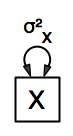
The model estimates the mean and the variance of the variable X. We call this model saturated because there is a free parameter corresponding to each and every observed statistic. Here we have covariance matrix input only, so we can estimate one variance. Below is the path diagram and the complete script:
require(OpenMx)

#example 1: Saturated Model with Cov Matrices and Path-Style Input
univSatModel1 <- mxModel("univSat1",
            type="RAM",
    manifestVars= selVars,
    mxPath(
        from=c("X"),
        arrows=2,
        free=T,
        values=1,
        lbound=.01,
        labels="vX"
    ),
    mxData(
        observed=var(testData),
        type="cov",
        numObs=1000
    )
)
Each of of the commands are discussed separately beside excerpts of the OpenMx code. We use the mxModel command to specify the model. Its first argument is a name. All arguments are separated by commas.
univSatModel1 <- mxModel("univSat1",
When using the path specification, it is easiest to work from an existing path diagram. Assuming you are familiar with path analysis (for those who are not, there are several excellent introductions, see refs), we have a box for the observed/manifest variable x, specified with the manifestVars argument, and one double headed arrow on the box to represent its variance, specified with the mxPath command. The mxPath command indicates where the path originates ( from=) and where it ends (to). If the to= argument is omitted, the path ends at the same variable where it started. The arrows argument distinguishes one-headed arrows (if arrows=1) from two-headed arrows (if arrows=2). The free command is used to specify which elements are free or fixed with a TRUE or FALSE option. If the mxPath command creates more than one path, a single T implies that all paths created here are free. If some of the paths are free and others fixed, a list is expected. The same applies for the values command which is used to assign starting values or fixed final values, depending on the corresponding ‘free’ status. Optionally, lower and upper bounds can be specified (using lbound and ubound, again generally for all the paths or specifically for each path). Labels can also be assigned using the labels command which expects as many labels (in quotes) as there are elements.
        type="RAM",
manifestVars=selVars,

mxPath(
    from=c("X"),
    arrows=2,
    free=T,
    values=1,
    lbound=.01,
    labels="vX"
),
We specify which data the model is fitted to with the mxData command. Its first argument, observed=, reads in the data from an R matrix or data.frame, with the type= given in the second argument. Given we read a covariance matrix here, we use the var() function (as there is no covariance for a single variable). When summary statistics are used as input, the number of observations (numObs=) needs to be supplied.
mxData(
    observed=var(testData),
    type="cov",
    numObs=1000
))
With the path specification, the ‘RAM’ objective function is used by default, as indicated by the type argument. Internally, OpenMx translates the paths into RAM notation in the form of the matrices A, S, and F [see refs].
Model Fitting
So far, we have specified the model, but nothing has been evaluated. We have ‘saved’ the specification in the object univSatModel1. This object is evaluated when we invoke the mxRun command with the object as its argument.
univSatFit1 <- mxRun(univSatModel1)
There are a variety of ways to generate output. We will promote the use of the mxEval command, which takes two arguments: an expression and a model name. The expression can be a matrix or algebra name defined in the model, new calculations using any of these matrices/algebras, the objective function, etc. We can then use any regular R function to generate derived fit statistics, some of which will be built in as standard. When fitting to covariance matrices, the saturated likelihood can be easily obtained and subtracted from the likelihood of the data to obtain a Chi-square goodness-of-fit.
EC1 <- mxEval(S, univSatFit1)   #univSatFit1[['S']]@values
LL1 <- mxEval(objective, univSatFit1)
SL1 <- univSatFit1@output$other$Saturated
Chi1 <- LL1-SL1
The output of these objects like as follows:
> EC1
             [,1]
    [1,] 1.062112
> LL1
             [,1]
    [1,] 1.060259
> SL1
    [1] 1.060259
> Chi1
                 [,1]
    [1,] 2.220446e-16
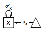
In addition to providing a covariance matrix as input data, we could add a means vector. As this requires a few minor changes, lets highlight those. We have one additional mxPath command for the means. In the path diagram, the means are specified by a triangle which as a fixed value of one, reflected in the from="one" argument, with the to= argument referring to the variable which mean is estimated. Note that paths for means are always single headed.
univSatModel1m <- mxModel(univSatModel1, name = "univSat1m",
    mxPath(
        from="one",
        to="X",
        arrows=1,
        free=T,
        values=0,
        labels="mX"
    ),
The other required change is in the mxData command, which now takes a fourth argument means for the vector of observed means from the data, calculated using the R mean command.
    mxData(
        observed=var(testData),
        type="cov",
        numObs=1000,
        means=colMeans(testData)
    )
)
When a mean vector is supplied and a parameter added for the estimated mean, the RAM matrices A, S and F are augmented with an M matrix which can be referred to in the output in a similar way as the expected variance before.
univSatFit1m <- mxRun(univSatModel1m)
EM1m <- mxEval(M, univSatFit1m)
Raw Data and Path-style Input
Instead of fitting models to summary statistics, it is now popular to fit models directly to the raw data and using full information maximum likelihood (FIML). Doing so requires specifying not only a model for the covariances, but also one for the means, just as in the case of fitting to covariance matrices and mean vectors described above. The path diagram for this model, now including means (path from triangle of value 1) is as follows:
The only change required is in the mxData command, which now takes either an R matrix or a data.frame with the observed data as first argument, and the type="raw" as the second argument.
mxData(
    observed=testData,
    type="raw"
)
A nice feature of OpenMx is that an existing model can be easily modified. So univSatModel1 can be modified as follows:
univRawModel1 <- mxModel(univSatModel1,
    mxData(
        observed=testData,
        type="raw"
    )
)
The resulting model can be run as usual using mxRun:
univRawFit1 <- mxRun(univSatModel1)
Note that the output now includes the expected means, as well as the expected covariance matrix and -2 x log-likelihood of the data.:
> EM2
               [,1]
    [1,] 0.01680498
> EC2
             [,1]
    [1,] 1.061049
> LL2
             [,1]
    [1,] 2897.135
Covariance Matrices and Matrix-style Input
The next example replicates these models using matrix-style coding. The code to specify the model includes four commands, (i) mxModel, (ii) mxMatrix, (iii) mxData and (iv) mxMLObjective.
Starting with the model fitted to the summary covariance matrix, we need to create a matrix for the expected covariance matrix using the mxMatrix command. The first argument is its type, symmetric for a covariance matrix. The second and third arguments are the number of rows (nrow) and columns (ncol) – one for a univariate model. The free and values parameters work as in the path specification. If only one element is given, it is applied to all elements of the matrix. Alternatively, each element can be assigned its free/fixed status and starting value with a list command. Note that in the current example, the matrix is a simple 1x1 matrix, but that will change rapidly in the following examples. The mxData is identical to that used in path stlye models. A different objective function is used, however, namely the mxMLObjective command which takes two arguments, covariance to hold the expected covariance matrix (which we specified above using mxMatrix as expCov), and dimnames which allow the mapping of the observed data to the expected covariance matrix, i.e. the model.
univSatModel3 <- mxModel("univSat3",
    mxMatrix(
        type="Symm",
        nrow=1,
        ncol=1,
        free=T,
        values=1,
        name="expCov"
    ),
    mxData(
        observed=var(testData),
        type="cov",
        numObs=1000
    ),
    mxMLObjective(
        covariance="expCov",
        dimnames=selVars
    )
)

univSatFit3 <- mxRun(univSatModel3)
A means vector can also be added as the fourth argument of the mxData command. When means are requested to be modeled, a second mxMatrix command is required to specify the vector of expected means. In this case a matrix of type='Full', with 1 row and column, is assigned free=T with start value 0, and the name expMean. The second change is an additional argument mean to the mxMLObjective function for the expected mean, here expMean.
mxMatrix(
    type="Full",
    nrow=1,
    ncol=1,
    free=TRUE,
    values=0,
    name="expMean"
)
mxData(
    observed=var(testData),
    type="cov",
    numObs=1000,
    means=colMeans(testData)
)
mxMLObjective(
    covariance="expCov",
    means="expMean",
    dimnames=selVars
)
Raw Data and Matrix-style Input
Finally, if we want to use the matrix specification with raw data, we specify matrices for the means and covariances using mxMatrix(). The mxData command now, however takes a matrix (or data.frame) of raw data and the mxFIMLObjective function replaces mxMLObjective to evaluate the likelihood of the data using FIML (Full Information Maximum Likelihood). This function takes three arguments: the expected covariance matrix covariance; the expected mean vector, means; and a third for the dimnames.
univSatModel4 <- mxModel("univSat4",
    mxMatrix(
        type="Symm",
        nrow=1,
        ncol=1,
        free=T,
        values=1,
        name="expCov"
    ),
    mxMatrix(
        type="Full",
        nrow=1,
        ncol=1,
        free=T,
        values=0,
        name="expMean"
    ),
    mxData(
        observed=testData,
        type="raw"
    ),
    mxFIMLObjective(
        covariance="expCov",
        means="expMean",
        dimnames=selVars
    )
)
Note that the output generated for the paths and matrices specification are completely equivalent.
Bivariate Saturated Model
Rarely will we analyze a single variable. As soon as a second variable is added, not only can we estimate both means and variances, but also a covariance between the two variables, as shown in the following path diagram:
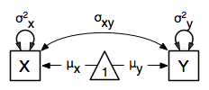
The path diagram for our bivariate example includes two boxes for the observed variables ‘X’ and ‘Y’, each with a two-headed arrow for the variance of each variables. We also estimate a covariance between the two variables with the two-headed arrow connecting the two boxes. The optional means are represented as single-headed arrows from a triangle to the two boxes.
Data
The data used for the example were generated using the multivariate normal function (mvrnorm in the R package MASS). We have simulated data on two variables named ‘X’ and ‘Y’ with means of zero, variances of one and a covariance of 0.5 using the following R code, and saved is as testData. Note that we can now use the R function cov to generate the observed covariance matrix.
#Simulate Data
require(MASS)
set.seed(200)
rs=.5
xy <- mvrnorm (1000, c(0,0), matrix(c(1,rs,rs,1),2,2))
testData <- xy
selVars <- c('X','Y')
dimnames(testData) <- list(NULL, selVars)
summary(testData)
cov(testData)
Model Specification
The mxPath commands look as follows. The first one specifies two-headed arrows from X and Y to themselves. This command now generates two free parameters, each with start value of 1 and lower bound of .01, but with a different label indicating that these are separate free parameters. Note that we could test whether the variances are equal by specifying a model with the same label for the two variances and comparing it with the current model. The second mxPath command specifies a two-headed arrow from X to Y for the covariance, which is also assigned ‘free’ and given a start value of .2 and a label.
mxPath(
    from=c("X", "Y"),
    arrows=2,
    free=T,
    values=1,
    lbound=.01,
    labels=c("varX","varY")
)
mxPath(
    from="X",
    to="Y",
    arrows=2,
    free=T,
    values=.2,
    lbound=.01,
    labels="covXY"
)
When observed means are included in addition to the observed covariance matrix, we add an mxPath command with single-headed arrows from one to the variables to represent the two means.
mxPath(
    from="one",
    to=c("X", "Y"),
    arrows=1,
    free=T,
    values=.01,
    labels=c("meanX","meanY")
)
Changes required for fitting to raw data are to the mxData command to read in the data directly with type=raw.
Using matrices instead of paths, our mxMatrix command for the expected covariance matrix now specifies a 2x2 matrix with all elements free. Start values have to be given only for the unique elements (diagonal elements plus upper or lower diagonal elements), in this case we provide a list with values of 1 for the variances and 0.5 for the covariance
mxMatrix(
    type="Symm",
    nrow=2,
    ncol=2,
    free=T,
    values=c(1,0.5,1),
    name="expCov"
)
The optional expected means command specifies a 1x2 row vector with two free parameters, each given a 0 start value.
mxMatrix(
    type="Full",
    nrow=1,
    ncol=2,
    free=T,
    values=c(0,0),
    name="expMean"
)
Combining these two mxMatrix commands with the raw data, specified in the mxData command and the mxFIMLObjective command with the appropriate arguments is all that is needed to fit a saturated bivariate model. So far, we have specified the expected covariance matrix directly as a symmetric matrix. However, this may cause optimization problems as the matrix could become not positive-definite which would prevent the likelihood to be evaluated. To overcome this problem, we can use a Cholesky decomposition of the expected covariance matrix instead, by multiplying a lower triangular matrix with its transpose. To obtain this, we use a mxMatrix command and specify type="Lower". We then use an mxAlgebra command to multiply this matrix, named Chol with its transpose (R function t()).
mxMatrix(
    type="Lower",
    nrow=2,
    ncol=2,
    free=T,
    values=.5,
    name="Chol"
)
mxAlgebra(
    Chol %*% t(Chol),
    name="expCov",
)
The following sections describe OpenMx examples in detail beginning with regression, factor analysis, time series analysis, multiple group models, including twin models, and analysis using definition variables. Each is presented in both path and matrix styles and where relevant, contrasting data input from covariance matrices versus raw data input are also illustrated. Additional examples will be added as they are implemented in OpenMx.