Introduction
Tutorial
Prerequisites
Congratulations! You have decided to check out OpenMx, the open source version of the statistical modeling package Mx, rewritten in R. Before we get started, let’s make sure you have the software installed and ready to go. You need:
Simple OpenMx Script
We will start by showing some of the main features of OpenMx using simple examples. For those familiar with Mx, it is basically a matrix interpreter combined with a numerical optimizer to allow fitting statistical models. Of course you do not need OpenMx to perform matrix algebra as that can already be done in R. However, to accommodate flexible statistical modeling of the type of models typically fit in Mx, Mplus or other SEM packages, special kinds of matrices and functions are required which are bundled in OpenMx. We will introduce key features of OpenMx using a matrix algebra example. Remember that R is object-oriented, such that the results of operations are objects, rather than just matrices, with various properties/characteristics attached to them. We will describe the script line by line; a link to the complete script is here.
Say, we want to create two matrices, A and B, each of them a ‘Full’ matrix with 3 rows and 1 column and with the values 1, 2 and 3, as follows:
![\begin{eqnarray*}
A = \left[ \begin{array}{r} 1 \\ 2 \\ 3 \\ \end{array} \right]
& B = \left[ \begin{array}{r} 1 \\ 2 \\ 3 \\ \end{array} \right]
\end{eqnarray*}](_images/math/7247d6af29b3339c76ee9ee437ad2aa54bbc0cc9.png)
we use the mxMatrix command, and define the type of the matrix (type=), number of rows (nrow=) and columns (ncol=), its specifications (free=) and starting values (values=), optionally labels (labels=), upper (ubound=) and lower (lbound=) bounds>, and a name (name=). The matrix A will be stored as the object ‘A’.
mxMatrix(
    type="Full",
    nrow=3,
    ncol=1,
    values=c(1,2,3),
    name='A'
)
mxMatrix(
    type="Full",
    nrow=3,
    ncol=1,
    values=c(1,2,3),
    name='B'
)
Assume we want to calculate the (1) the sum of the matrices A and B, (2) the element by element multiplication (Dot product) of A and B, (3) the transpose of matrix A, and the (4) outer and (5) inner products of the matrix A, using regular matrix multiplication, i.e.:
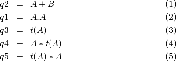
we invoke the mxAlgebra command which performs an algebra operation between previously defined matrices. Note that in R, regular matrix multiplication is represented by \%*\% and dot multiplication as *. We also assign the algebras a name to refer back to them later:
mxAlgebra(
        A + B,
        name='q1'
)
mxAlgebra(
        A * A,
        name='q2'
)
mxAlgebra(
        t(A),
        name='q3'
)
mxAlgebra(
        A %*% t(A),
        name='q4'
)
mxAlgebra(
        t(A) %*% A,
        name='q5'
)
For the algebras to be evaluated, they become arguments of the mxModel command, as do the defined matrices, each separated by comma’s. The model, which is here given the name ‘algebraExercises’, is then executed by the mxRun command, as shown in the full code below:
require(OpenMx)

algebraExercises <- mxModel(
    mxMatrix(type="Full", nrow=3, ncol=1, values=c(1,2,3), name='A'),
    mxMatrix(type="Full", nrow=3, ncol=1, values=c(1,2,3), name='B'),
    mxAlgebra(A+B, name='q1'),
            mxAlgebra(A*A, name='q2'),
            mxAlgebra(t(A), name='q3'),
    mxAlgebra(A%*%t(A), name='q4'),
    mxAlgebra(t(A)%*%A, name='q5'))

answers <- mxRun(algebraExercises)
answers@algebras
result <- mxEval(list(q1,q2,q3,q4,q5),answers)
As you notice, we added some lines at the end to generate the desired output. The resulting matrices and algebras are stored in answers; we can refer back to them by specifying answers@matrices or answers@algebras. We can also calculate any additional quantities or perform extra matrix operations on the results using the mxEval command. For example, if we want to see all the answers to the questions in matrixAlgebra.R, the results would look like this:
[[1]]
        [,1]
[1,]    2
[2,]    4
[3,]    6

[[2]]
        [,1]
[1,]    1
[2,]    4
[3,]    9

[[3]]
        [,1] [,2] [,3]
[1,]    1    2    3

[[4]]
        [,1] [,2] [,3]
[1,]    1    2    3
[2,]    2    4    6
[3,]    3    6    9

[[5]]
        [,1]
[1,]   14
So far, we have introduced five new commands: mxMatrix, mxAlgebra, mxModel, mxRun and mxEval. These commands allow us to run a wide range of jobs, from simple matrix algebra to rather complicated SEM models. Let’s move to an example involving optimizing the likelihood of observed data.
Optimization Script
When collecting data to test a specific hypothesis, one of the first things one typically does is checking the basic descriptive statistics, such as the means, variances and covariances/correlations. We could of course use basic functions in R, i.e., meanCol(Data) or cov(Data) to perform these operations. However, if we want to test specific hypotheses about the data, for example, test whether the correlation between two variables is significantly different from zero, we need to compare the likelihood of the data when the correlation is freely estimated with the likelihood of the data when the correlation is fixed to zero. Let’s work through a specific example.
Say, we have collected data on two variables X and Y in 1000 individuals, and R descriptive statistics has shown that the correlation between them is 0.5. For the sake of this example, we used another built-in function in the R package MASS, namely mvrnorm, to generate multivariate normal data for 1000 individuals with means of 0.0, variances of 1.0 and a correlation (rs) of 0.5 between X and Y. Note the that first argument of mvrnorm is the sample size, the second the vector of means, and the third the covariance matrix to be simulated. We save the data in the object xy and create a vector of labels for the two variables in selVars which is used in the dimnames statement later on. The R functions summary() and cov() are used to verify that the simulations appear OK.
#Simulate Data
require(MASS)
set.seed(200)
rs=.5
xy <- mvrnorm (1000, c(0,0), matrix(c(1,rs,rs,1),2,2))
testData <- xy
selVars <- c('X','Y')
dimnames(testData) <- list(NULL, selVars)
summary(testData)
cov(testData)
To evaluate the likelihood of the data using SEM, we estimate a saturated model with free means, free variances and a covariance. Let’s start with specifying the mean vector. We use the mxMatrix command, provide the type, here Full, the number of rows and columns, respectively 1 and 2, the specification of free/fixed parameters, the starting values, the dimnames and a name. Given all the elements of this 1x2 matrix are free, we can use free=True. The starting values are provided using a list, i.e. c(0,0). The dimnames are a type of label that is required to recognize the expected mean vector and expected covariance matrix and match up the model with the data. For a mean vector, the first element is NULL given mean vectors always have one row. The second element of the list should have the labels for the two variables c('X','Y') which we have previously assigned to the object selVars. Finally, we are explicit in naming this matrix expMean. Thus the matrix command looks like this. Note the soft tabs to improve readability.
bivCorModel <- mxModel("bivCor",
    mxMatrix(
        type="Full",
        nrow=1,
        ncol=2,
        free=TRUE,
        values=c(0,0),
        name="expMean"
    ),
Next, we need to specify the expected covariance matrix. As this matrix is symmetric, we could estimate it directly as a symmetric matrix. However, to avoid solutions that are not positive definite, we will use a Cholesky decomposition. Thus, we specify a lower triangular matrix (matrix with free elements on the diagonal and below the diagonal, and zero’s above the diagonal), and multiply it with its transpose to generate a symmetric matrix. We will use a mxMatrix command to specify the lower triangular matrix and a mxAlgebra command to set up the symmetric matrix. The matrix is a 2x2 free lower matrix with c('X','Y') (previously defined as selVars) as dimnames for the rows and columns, and the name “Chol”. We can now refer back to this matrix by its name in the mxAlgebra statement. We use a regular multiplication of Chol with its transpose t(Chol), and name this as “expCov”.
mxMatrix(
    type="Lower",
    nrow=2,
    ncol=2,
    free=TRUE,
    values=.5,
    name="Chol"
),
mxAlgebra(
    expression=Chol %*% t(Chol),
    name="expCov"
),
Now that we have specified our ‘model’, we need to supply the data. This is done with the mxData command. The first argument includes the actual data, in the type given by the second argument. Type can be a covariance matrix (cov), a correlation matrix (cor), a matrix of cross-products (sscp) or raw data (raw). We will use the latter option and read in the raw data directly from the simulated dataset testData.
mxData(
    observed=testData,
    type="raw"
),
Next, we specify which objective function we wish to use to obtain the likelihood of the data. Given we fit to the raw data, we use the full information maximum likelihood (FIML) objective function mxFIMLObjective. Its arguments are the expected covariance matrix, generated using the mxMatrix and mxAlgebra commands as “expCov”, and the expected means vectors, generated using the mxMatrix command as “expMeans”.
mxFIMLObjective(
    covariance="expCov",
    means="expMean",
    dimnames=selVars)
)
All these elements become arguments of the mxModel command, seperated by comma’s. The first argument can be a name, as in this case “bivCor” or another model (see below). The model is saved in an object ‘bivCorModel’. This object becomes the argument of the mxRun command, which evaluates the model and provides output - if the model ran successfully - using the following command.
bivCorFit <- mxRun(bivCorModel)
We can request various parts of the output to inspect by referring to them by the name of the object resulting from the mxRun command, i.e. bivCorFit, followed by the name of the objects corresponding to the expected mean vector, i.e. [['ExpMean']], and covariance matrix, i.e. [['ExpCov']], in quotes and double square brackets, followed by @values. The command mxEval can also be used to extract relevant information, such as the likelihood, (objective) where the first argument of the command is the object of interest and the second the object obtaining the results.
EM <- bivCorFit[['expMean']]@values
EC <- bivCorFit[['expCov']]@values
LL <- mxEval(objective,bivCorFit);
These commands generate the following output:
EM
          X            Y
[1,] 0.03211646 -0.004883803

EC
          X         Y
X 1.0092847 0.4813501
Y 0.4813501 0.9935387

LL
         [,1]
[1,] 5415.772
Standard lists of parameter estimates and goodness-of-fit statistics can also be obtained with the summary command.
> summary(bivCorFit)
       X                   Y
 Min.   :-2.942561   Min.   :-3.296159
 1st Qu.:-0.633711   1st Qu.:-0.596177
 Median :-0.004139   Median :-0.010538
 Mean   : 0.032116   Mean   :-0.004884
 3rd Qu.: 0.739236   3rd Qu.: 0.598326
 Max.   : 4.173841   Max.   : 4.006771

  name  matrix row col parameter estimate error estimate
1 <NA> expMean   1   1        0.032116456     0.02228409
2 <NA> expMean   1   2       -0.004883803     0.02235021
3 <NA>    Chol   1   1        1.004631642     0.01575904
4 <NA>    Chol   2   1        0.479130899     0.02099642
5 <NA>    Chol   2   2        0.874055066     0.01376876

Observed statistics:  2000
Estimated parameters:  5
Degrees of freedom:  1995
-2 log likelihood:  5415.772
Saturated -2 log likelihood:
Chi-Square:
p:
AIC (Mx):  1425.772
BIC (Mx):  -4182.6
adjusted BIC:
RMSEA:  0
If we want to test whether the covariance/correlation is significantly different from zero, we could fit a submodel and compare it with the previous saturated model. Given that this model is essentially the same as the original, except for the covariance, we create a new mxModel (named ‘bivCorModelSub) with as first argument the old model (named ‘bivCorModel). Then we only have to specify the matrix that needs to be changed, in this case the lower triangular matrix becomes essentially a diagonal matrix, obtained by fixing the off-diagonal elements to zero in the free and values arguments
#Test for Covariance=Zero
bivCorModelSub <-mxModel(bivCorModel,
    mxMatrix(
                    type="Diag",
                    nrow=2,
                    ncol=2,
                    free=TRUE,
                    dimnames=list(selVars, selVars),
                    name="Chol"
    )
We can output the same information as for the saturated job, namely the expected means and covariance matrix and the likelihood, and then use R to calculate other statistics, such as the Chi-square goodness-of-fit.
bivCorFitSub <- mxRun(bivCorModelSub)
EMs <- mxEval(expMean, bivCorFitSub)
ECs <- mxEval(expCov, bivCorFitSub)
LLs <- mxEval(objective, bivCorFitSub)
Chi= LLs-LL;
LRT= rbind(LL,LLs,Chi); LRT
More in-depth Example
Now that you have seen the basics of OpenMx, let us walk through an example in more detail. We decided to use a twin model example for several reasons. Even though you may not have any background in behavior genetics or genetic epidemiology, the example illustrates a number of features you are likely to encounter at some stage. We will present the example in two ways: (i) path analysis representation, and (ii) matrix algebra representation. Both give exactly the same answer, so you can choose either one or both to get some familiarity with the two approaches.
We will not go into detail about the theory of this model, as that has been done elsewhere (refs). Briefly, twin studies rely on comparing the similarity of identical (monozygotic, MZ) and fraternal (dizygotic, DZ) twins to infer the role of genetic and environmental factors on individual differences. As MZ twins have identical genotypes, similarity between MZ twins is a function of shared genes, and shared environmental factors. Similarity between DZ twins is a function of some shared genes (on average they share 50% of their genes) and shared environmental factors. A basic assumption of the classical twin design is that the MZ and DZ twins shared environmental factors to the same extent.
The basic model typically fit to twin data from MZ and DZ twins reared together includes three sources of latent variables: additive genetic factors (A), shared environmental influences (C) and unique environmental factors (E), We can estimate these three sources of variance from the observed variances, the MZ and the DZ covariance. The expected variance is the sum of the three variance components (A + C + E). The expected covariance for MZ twins is (A + C) and that of DZ twins is (.5A + C). As MZ and DZ twins have different expected covariances, we have a multiple group model.
It has been standard in twin modeling to fit models to the raw data, as often data are missing on some co-twins. When using FIML, we also need to specify the expected means. There is no reason to expect that the variances are different for twin 1 and twin 2, neither are the means for twin 1 and twin 2 expected to differ. This can easily be verified by fitting submodels to the saturated model, prior to fitting the *ACE* model.
Let us start by simulating the data following by fitting a series of models. The code. includes both the twin data simulation and several OpenMx scripts to analyze the data. We will describe each of the parts in turn and include the code for the specific part in the code blocks.
First, we simulate twin data using the mvrnorm R function. If the additive genetic factors (A) account for 50% of the total variance and the shared environmental factors (C) for 30%, thus leaving 20% explained by specific environmental factors (E), then the expected MZ twin correlation is a^2 + c^2 or 0.8 in this case, and the expected DZ twin correlation is 0.65, calculated as .5*a^2 + c^2. We simulate 1000 pairs of MZ and DZ twins each with zero means and a correlation matrix according to the values listed above. We run some basic descriptive statistics on the simulated data, using regular R functions.
require(OpenMx)

    require(MASS)
    set.seed(200)
    a2<-0.5         #Additive genetic variance component (a squared)
    c2<-0.3         #Common environment variance component (c squared)
    e2<-0.2         #Specific environment variance component (e squared)
    rMZ <- a2+c2
    rDZ <- .5*a2+c2
    MZ <- mvrnorm (1000, c(0,0), matrix(c(1,rMZ,rMZ,1),2,2))
    DZ <- mvrnorm (1000, c(0,0), matrix(c(1,rDZ,rDZ,1),2,2))

    selVars <- c('t1','t2')
    dimnames(DataMZ) <- list(NULL,selVars)
    dimnames(DataDZ) <- list(NULL,selVars)
    summary(DataMZ)
    summary(DataDZ)
    colMeans(DataMZ,na.rm=TRUE)
    colMeans(DataDZ,na.rm=TRUE)
    cov(DataMZ,use="complete")
    cov(DataDZ,use="complete")
We typically start with fitting a saturated model, estimating means, variances and covariances separately by order of the twins (twin 1 vs twin 2) and by zygosity (MZ vs DZ pairs), to establish the likelihood of the data. This is essentially similar to the optimization script discussed above, except that we now have two variables (same variable for twin 1 and twin 2) and two groups (MZ and DZ). Thus, the saturated model will have two matrices for the expected means of MZs and DZs, and two for the expected covariances, generated from multiplying a lower triangular matrix with its transpose. The raw data are read in using the mxData command, and the corresponding objective function mxFIMLObjective applied.
mxModel("MZ",
        mxMatrix(
                type="Full",
                nrow=1,
                ncol=2,
                free=TRUE,
                values=c(0,0),
                dimnames=list(NULL,selVars),
                name="expMeanMZ"),
        mxMatrix(
                type="Lower",
                nrow=2,
                ncol=2,
                free=TRUE
                values=.5,
                dimnames=list(NULL, selVars),
                name="CholMZ"),
        mxAlgebra(
                CholMZ %*% t(CholMZ),
                name="expCovMZ",
                dimnames=list(selVars, selVars)),
        mxData(
                DataMZ,
                type="raw"),
        mxFIMLObjective(
                "expCovMZ",
                "expMeanMZ"))
Note that the mxModel statement for the DZ twins is almost identical to that for MZ twins, except for the names of the objects and data. If the arguments to the OpenMx command are given in the default order (see i.e. ?mxMatrix to go to the help/reference page for that command), then it is not necessary to include the name of the argument. Given we skip a few optional arguments, the argument names dimnames= and name= are included to refer to the right arguments. For didactic purposes, we prefer the formatting used for the MZ group, with soft tabs and each argument on a separate line, etc. (see list of formatting rules). However, the experienced user may want to use a more compact form, as the one used for the DZ group.
mxModel("DZ",
    mxMatrix("Full", 1, 2, T, c(0,0), dimnames=list(NULL, selVars), name="expMeanDZ"),
    mxMatrix("Lower", 2, 2, T, .5, dimnames=list(NULL, selVars), name="CholDZ"),
    mxAlgebra(CholDZ %*% t(CholDZ), name="expCovDZ", dimnames=list(selVars, selVars)),
    mxData(DataDZ, type="raw"),
    mxFIMLObjective("expCovDZ", "expMeanDZ")),
The two models are then combined in a ‘super’model which includes them as arguments. Additional arguments are an mxAlgebra statement to add the objective funtions/likelihood of the two submodels. To evaluate them simultaneously, we use the mxAlgebraObjective with the previous algebra as its argument. The mxRun command is used to start optimization.
twinSatModel <- mxModel("twinSat",
        mxModel("MZ",
                mxMatrix("Full", 1, 2, T, c(0,0), dimnames=list(NULL, selVars), name="expMeanMZ"),
                mxMatrix("Lower", 2, 2, T, .5, dimnames=list(NULL, selVars), name="CholMZ"),
                mxAlgebra(CholMZ %*% t(CholMZ), name="expCovMZ", dimnames=list(selVars, selVars)),
                mxData(DataMZ, type="raw"),
                mxFIMLObjective("expCovMZ", "expMeanMZ")),
        mxModel("DZ",
                mxMatrix("Full", 1, 2, T, c(0,0), dimnames=list(NULL, selVars), name="expMeanDZ"),
                mxMatrix("Lower", 2, 2, T, .5, dimnames=list(NULL, selVars), name="CholDZ"),
                mxAlgebra(CholDZ %*% t(CholDZ), name="expCovDZ", dimnames=list(selVars, selVars)),
                mxData(DataDZ, type="raw"),
                mxFIMLObjective("expCovDZ", "expMeanDZ")),
        mxAlgebra(MZ.objective + DZ.objective, name="twin"),
        mxAlgebraObjective("twin"))
twinSatFit <- mxRun(twinSatModel)
It is always helpful/advised to check the model specifications before interpreting the output. Here we are interested in the values for the expected mean vectors and covariance matrices, and the goodness-of-fit statistics, including the likelihood, degrees of freedom, and any other derived indices.
ExpMeanMZ <- mxEval(MZ.expMeanMZ, twinSatFit)
ExpCovMZ <- mxEval(MZ.expCovMZ, twinSatFit)
ExpMeanDZ <- mxEval(DZ.expMeanDZ, twinSatFit)
ExpCovDZ <- mxEval(DZ.expCovDZ, twinSatFit)
LL_Sat <- mxEval(objective, twinSatFit)
Before we move on to fit the ACE model to the same data, we may want to test some of the assumptions of the twin model, i.e. that the means and variances are the same for twin 1 and twin 2, and that they are the same for MZ and DZ twins. This can be done as an omnibus test, or stepwise. Let us start by equating the means for both twins, separately in the two groups. We accomplish this by using the same label (just one label which will be reused by R) for the two free parameters for the means per group. As the majority of the previous script stays the same, we start by copying the old model into a new one. We then include the arguments of the model that require a change.
twinSatModelSub1 <- mxModel(twinSatModel,
    mxModel("MZ",
        mxMatrix("Full", 1, 2, T, 0, "mMZ", dimnames=list(NULL, selVars), name="expMeanMZ"),
    mxModel("DZ",
        mxMatrix("Full", 1, 2, T, 0, "mDZ", dimnames=list(NULL, selVars), name="expMeanDZ"))
twinSatFitSub1 <- mxModel(twinSatModelSub1)
If we want to test if we can equate both means and variances across twin order and zygosity at once, we will end up with the following specification. Note that we use the same label across models for elements that need to be equated.
twinSatModelSub2 <- mxModel(twinSatModelSub1,
    mxModel("MZ",
        mxMatrix("Full", 1, 2, T, 0, "mean", dimnames=list(NULL, selVars), name="expMeanMZ"),
        mxMatrix("Lower", 2, 2, T, .5, labels= c("var","MZcov","var"),
            dimnames=list(NULL, selVars), name="CholMZ"),
    mxModel("DZ",
        mxMatrix("Full", 1, 2, T, 0, "mean", dimnames=list(NULL, selVars), name="expMeanDZ"),
        mxMatrix("Lower", 2, 2, T, .5, labels= c("var","DZcov","var"),
            dimnames=list(NULL, selVars), name="CholDZ"))
twinSatFitSub2 <- mxRun(twinSatModelSub2)
We can compare the likelihood of this submodel to that of the fully saturated model or the previous submodel using the results from mxEval commands with regular R algebra. A summary of the model parameters, estimates and goodness-of-fit statistics can also be obtained using summary(twinSatFit).
LL_Sat <- mxEval(objective, twinSatFit)
LL_Sub1 <- mxEval(objective, twinSatFitSub1)
LRT1= LL_Sub1 - LL_Sat
LL_Sub2 <- mxEval(objective, twinSatFitSub1)
LRT2= LL_Sub2 - LL_Sat
Now, we are ready to specify the ACE model to test which sources of variance significantly contribute to the phenotype and estimate their best value. The structure of this script is going to mimic that of the saturated model. The main difference is that we no longer estimate the variance-covariance matrix directly, but express it as a function of the three sources of variance, A, C and E. As the same sources are used for the MZ and the DZ group, the matrices which will represent them are part of the ‘super’model. As these sources are variances, which need to be positive, we typically use a Cholesky decomposition of the standard deviations (and effectively estimate a rather then a^2, see later for more in depth coverage). Thus, we specify three separate matrices for the three sources of variance using the mxMatrix command and ‘calculate’ the variance components with the mxAlgebra command. Note that there are a variety of ways to specify this model, we have picked one that corresponds well to previous Mx code, and has some intuitive appeal.
#Specify ACE Model
twinACEModel <- mxModel("twinACE",
        mxMatrix("Full", 1, 2, T, 20, "mean", dimnames=list(NULL, selVars), name="expMean"),
        # Matrix expMean for expected mean vector for MZ and DZ twins
        mxMatrix("Full", nrow=1, ncol=1, free=TRUE, values=.6, label="a", name="X"),
        mxMatrix("Full", nrow=1, ncol=1, free=TRUE, values=.6, label="c", name="Y"),
        mxMatrix("Full", nrow=1, ncol=1, free=TRUE, values=.6, label="e", name="Z"),
        # Matrices X, Y, and Z to store the a, c, and e path coefficients
        mxMatrix("Full", nrow=1, ncol=1, free=FALSE, values=.5, name="h"),
        mxAlgebra(X * t(X), name="A"),
        mxAlgebra(Y * t(Y), name="C"),
        mxAlgebra(Z * t(Z), name="E"),
        # Matrixes A, C, and E to compute A, C, and E variance components
        mxAlgebra(rbind(cbind(A+C+E   , A+C),
        cbind(A+C     , A+C+E)), dimnames = list(selVars, selVars), name="expCovMZ"),
        # Matrix expCOVMZ for expected covariance matrix for MZ twins
        mxAlgebra(rbind(cbind(A+C+E   , h%x%A+C),
        cbind(h%x%A+C , A+C+E)), dimnames = list(selVars, selVars), name="expCovDZ"),
        # Matrix expCOVMZ for expected covariance matrix for DZ twins
        mxModel("MZ",
                mxData(DataMZ, type="raw"),
                mxFIMLObjective("twinACE.expCovMZ", "twinACE.expMean")),
        mxModel("DZ",
                mxData(DataDZ, type="raw"),
                mxFIMLObjective("twinACE.expCovDZ", "twinACE.expMean")),
        mxAlgebra(MZ.objective + DZ.objective, name="twin"),
        mxAlgebraObjective("twin"))
twinACEFit <- mxRun(twinACEModel)
Relevant output can be generate with print or summary statements or specific output can be requested using the mxEval command. Typically we would compare this model back to the saturated model to interpret its goodness-of-fit. Parameter estimates are obtained and can easily be standardized. A typical analysis would likely include the following output.
LL_ACE <- mxEval(objective, twinACEFit)
LRT_ACE= LL_ACE - LL_Sat

#Retrieve expected mean vector and expected covariance matrices
        MZc <- mxEval(expCovMZ, twinACEFit)
        DZc <- mxEval(expCovDZ, twinACEFit)
        M   <- mxEval(expMean, twinACEFit)
#Retrieve the A, C, and E variance components
        A <- mxEval(A, twinACEFit)
        C <- mxEval(C, twinACEFit)
        E <- mxEval(E, twinACEFit)
#Calculate standardized variance components
        V <- (A+C+E)
        a2 <- A/V
        c2 <- C/V
        e2 <- E/V
#Build and print reporting table with row and column names
        ACEest <- rbind(cbind(A,C,E),cbind(a2,c2,e2))
        ACEest <- data.frame(ACEest, row.names=c("Variance Components","Standardized VC"))
        names(ACEest)<-c("A", "C", "E")
        ACEest; LL_ACE; LRT_ACE
Similarly to fitting submodels from the saturated model, we typically fit submodels of the ACE model to test the significance of the sources of variance. One example is testing the significance of shared environmental factors by dropping the free parameter for c (fixing it to zero). We call up the previous model and include the new specification for the matrix to be changed, and rerun.
twinAEModel <- mxModel(twinACEModel,
    mxMatrix("Full", nrow=1, ncol=1, free=F, values=0, label="c", name="Y"))
twinAEFit <- mxRun(twinAEModel)
We discuss twin analysis examples in more detail in the example code.
Two Model Styles - Two Data Styles
In this first detailed example, we introduce the different styles available to specify models and data. There are two main approaches to specifying models: (i) paths specification and (ii) matrix specification. We will go through all the examples in both approaches, so you can choose which fits your style better, or check them both out to get a sense of their advantage/disadvantages. The ‘path specification’ model style translates path diagrams into OpenMx code; the ‘matrix specification’ model style relies on matrices and matrix algebra to produce OpenMx code. For each of the two approaches, the data may come in (a) summary format, i.e. covariance matrices and possibly means, or (b) raw data format. We will illustrate both, as arguments of functions may differ. Thus, we will here describe the same example four different ways:
- i.a Path Specification - Covariance Matrices
- i.b Path Specification - Raw Data
- ii.a Matrix Specification - Covariance Matrices
- ii.b Matrix Specification - Raw Data
Our first example is fitting a simple model to one variable to estimate its mean and variance. This is also referred to as fitting a saturated model. We start with a univariate example, and also work through a bivariate example which differs in minor ways from the univariate one, as it forms the basis for later examples.
Univariate Saturated Model
The four versions of univariate example are available in the following files:
- UnivariateSaturated_PathCov.R
- UnivariateSaturated_PathRaw.R
- UnivariateSaturated_MatrixCov.R
- UnivariateSaturated_MatrixRaw.R
- UnivariateSaturated.R
The last file includes all four example in one. The bivariate examples are available in the following files:
- BivariateSaturated_PathCov.R
- BivariateSaturated_PathRaw.R
- BivariateSaturated_MatrixCov.R
- BivariateSaturated_MatrixRaw.R
- BivariateSaturated_MatrixCovCholesky.R
- BivariateSaturated_MatrixRawCholesky.R
- BivariateSaturated.R
Note that we have additional version of the matrix-style examples which use a Cholesky decomposition to estimate the expected covariance matrices, which is preferred to directly estimation the symmetric matrices.
Data
To avoid reading in data from an external file, we simulate a simple dataset directly in R, and use some of its great capabilities. As this is not an R manual, we just provide the code here with minimal explanation.
#Simulate Data
set.seed(100)
x <- rnorm (1000, 0, 1)
testData <- as.matrix(x)
selVars <- c("X")
dimnames(testData) <- list(NULL, selVars)
summary(testData)
mean(testData)
var(testData)
The first line is a comment (starting with a #). We set a seed for the simulation so that we generate the same data each time and get a reproducible answer. We then create a variable x for 1000 subjects, with mean of 0 and a variance of 1, using the normal distribution function. We read the data in as a matrix into an object ‘testData’ and give the variable a name “X” using the ‘dimnames’ command. We can easily produce some descriptive statistics in R using built-in functions ‘summary’, ‘mean’ and ‘var’, just to make sure the data look like what we expect.
Covariance Matrices and Path-style Input
Model Specification
We call this model saturated because there is a free parameter corresponding to each and every observed statistic. Here we have covariance matrix input only, so we can estimate one variance. We use the mxModel command to specify the model. Its first argument is a name. All arguments are separated by commas.
univSatModel1 <- mxModel("univSat1",
When using the path specification, it is easiest to have a matching path diagram. Assuming you are familiar with path analysis (for those who are not, there are several excellent introductions, see refs), we have a box for the observed/manifest variable x, specified with the manifestVars argument, and one double arrow on the box to represent its variance, specified with the mxPath command. The mxPath command indicates where the path originates: from= and where it ends: to. If the to= argument is omitted, the path ends at the same variable where it started. The arrows argument distinguished with one-head arrows (if arrows=1) or two-headed arrows (if arrows=2). The free command is used to specify which elements are free or fixed with a ‘TRUE’ or ‘FALSE’ option. If the mxPath command creates more than one path, a single ‘T’ implies that all paths created here are free. If some of the paths are free and others fixed, a list is expected. The same applies for values command which is used to assign starting values or fixed final values, depending on the corresponding ‘free’ status. Optionally, lower and upper bounds can be specified (using lbound and ubound, again generally for all the paths or specifically for each path). Labels can also be assigned using the labels command which expects as many labels (in quotes) as there are elements.
manifestVars=selVars ,

mxPath(
    from=c("X"),
    arrows=2,
    free=T,
    values=1,
    lbound=.01,
    labels="vX"
),
We specify which data the model is fitted to with the mxData command. Its first argument, matrix????, reads in the data from an R matrix or data.frame, with the type given in the second argument. Given we read a covariance matrix here, we use the ‘var’ function (as there is no covariance for a single variable). When summary statistics are used as input, the number of observations (numObs) needs to be supplied.
mxData(
    observed=var(testData),
    type="cov",
    numObs=1000
),
With the path specification, the ‘RAM’ objective function is used by default, as indicated by the type argument. Internally, OpenMx translates the paths into RAM notation in the form of the matrices A, S, and F [see ?]
    type="RAM"
)
Model Fitting
So far, we have specified the model, but nothing has been evaluated. We have ‘saved’ the specification in the object ‘univSatModel1’. This object is evaluated when we invoke the mxRun command with the object as its argument.
univSatFit1 <- mxRun(univSatModel1)
There are a variety of ways to generate output. We will promote the use of the mxEval command, which takes two arguments: an expression and a model name. The expression can be a matrix or algebra name defined in the model, new calculations using any of these matrices/algebras, the objective function, etc. We can then use any regular R function to generate derived fit statistics, some of which will be built in as standard. When fitting to covariance matrices, the saturated likelihood can be easily obtained and subtracted from the likelihood of the data to obtain a Chi-square goodness-of-fit. [How do we specify other$Saturated in mxEval?]
EC1 <- mxEval(S, univSatFit1)   #univSatFit1[['S']]@values
LL1 <- mxEval(objective, univSatFit1)
SL1 <- univSatFit1@output$other$Saturated
Chi1 <- LL1-SL1
The output of these objects like as follows:
> EC1
         [,1]
[1,] 1.062112
> LL1
         [,1]
[1,] 1.060259
> SL1
[1] 1.060259
> Chi1
             [,1]
[1,] 2.220446e-16
In addition to providing a covariance matrix as input data, we could use add a means vector. As this requires a few minor changes, lets highlight those. We have one additional mxPath command for the means. In the path diagram, the means are specified by a triangle which as a fixed value of one, reflected in the from="one" argument, with the to= argument referring to the variable which mean is estimated.
mxPath(
    from="one",
    to="X",
    arrows=1,
    free=T,
    values=0,
    labels="mX"
)
The other required change is in the mxData command, which now takes a fourth argument means for the vector of observed means from the data calculated using the R ‘mean’ command.
mxData(
    observed=matrix(var(testData),1,1),
    type="cov",
    numObs=1000,
    means=mean(testData)
)
When a mean vector is supplied and a parameter added for the estimated mean, the RAM matrices A, S and F are augmented with an M matrix which can be referred to in the output in a similar was as the expected variance before.
EM1m <- mxEval(M, univSatFit1m)
Raw Data and Path-style Input
Instead of fitting models to summary statistics, it is now popular to fit models directly to the raw data and using full information maximum likelihood (FIML). Doing so requires specifying not only a model for the covariances, but also one for the means, just as in the case of fitting to covariance matrices and mean vectors, described above. #With RAM path specification, and raw data input, OpenMx has a default model for the means, in which every observed variable has a free parameter for its mean [NB this should change in future versions to require means model]. The only change required is in the mxData command, which now takes either an R matrix or a data.frame with the observed data as first argument, and the type="raw" as the second argument.
mxData(
    observed=testData,
    type="raw"
)
A nice feature of OpenMx is that an existing model can be modified in any respect. So to change the above ‘univSatModel1’ can be effected this way:
univRawModel1 <- mxModel(univSatModel1,mxData(
        observed=testData,
        type="raw"
))
This model can be run as usual with an mxRun command: .. code-block:: r
univRawFit1 <- mxRun(univSatModel1)
Note The output generated from this model now includes the expected mean, the expected covariance matrix and -2 times the log-likelihood of the data.
> EM2
           [,1]
[1,] 0.01680498
> EC2
         [,1]
[1,] 1.061049
> LL2
         [,1]
[1,] 2897.135
Covariance Matrices and Matrix-style Input
We now specify essentially the same models with matrices. Starting with the model fitted to the summary covariance matrix, we need a specify one matrix for the expected covariance matrix. We use the mxMatrix command for this. The first argument is its type, which is symmetric for a covariance matrix. The second and third arguments are the number of rows (nrow) and columns (ncol). The free and values command work in the same way as in the path specification. If only one element is given, it is applied to all the elements in the matrix. Alternatively, each element can be assigned its free/fixed status and starting value with a list command. Note that in the current example, the matrix is a simple 1x1 matrix, but that will change rapidly in the following examples. The code to specify the model includes four commands, (i) mxModel, (ii) mxMatrix, (iii) mxData and (iv) mxMLObjective. The ``mxData is the same for paths and matrices specifications. A different objective function is used, namely the mxMLObjective command which takes one argument, the expression/name of the expected covariance matrix, which we specified in the mxMatrix command.
univSatModel3 <- mxModel("univSat3",
    mxMatrix(
        type="Symm",
        nrow=1,
        ncol=1,
        free=T,
        values=1,
        name="expCov"
    ),
    mxData(
        observed=var(testData),
        type="cov",
        numObs=1000
    ),
    mxMLObjective(
        "expCov", dimnames=selVars)
    )
univSatFit3 <- mxRun(univSatModel3)
A means vector can also be added here as part of the input summary statistics (as the fourth argument of the mxData command). In that case, a second mxMatrix command is used to specify the expected mean vector, which is of type ‘Full’, has 1 row and 1 column, is assigned ‘free’ with start value 0, dimnames for the column, and the name “expMean”. The second change is an additional argument to the mxMLObjective function for the expected mean, here “expMean”.
....
mxMatrix(
    type="Full",
    nrow=1,
    ncol=1,
    free=T,
    values=0,
    name="expMean"
),
mxData(
    observed=var(testData),
    type="cov",
    numObs=1000,
    means=mean(testData)
),
mxMLObjective(
    "expCov",
    "expMean",
    dimnames=selVars
)
Raw Data and Matrix-style Input
Finally, if we want to use the matrix specification with raw data, we again specify two matrices using the mxMatrix command, one for the expected covariance matrix and one for the expected mean vector, in the same way as before. The mxData command directly read the raw data from a matrix or data.frame and the mxFIMLObjective command is used to evaluate the likelihood of the data using FIML. This function also takes two arguments, one for the expected covariance matrix and one for the expected mean.
univSatModel4 <- mxModel("univSat4",
    mxMatrix(
        type="Symm",
        nrow=1,
        ncol=1,
        free=T,
        values=1,
        name="expCov"
    ),
    mxMatrix(
        type="Full",
        nrow=1,
        ncol=1,
        free=T,
        values=0,
        name="expMean"
    ),
    mxData(
        observed=testData,
        type="raw"
    ),
    mxFIMLObjective(
        "expCov",
        "expMean",
        dimnames=selVars)
    )
Note that the output generated for the paths and matrices specification are completely equivalent.
Bivariate Saturated Model
Rarely will we analyze a single variable. As soon as a second variable is added, not only can be then estimate two means and two variances, but also a covariance between the two variables.
Data
The data used for the example were generated using the multivariate normal function (mvrnorm in the R package MASS). We have simulated data on two variables named ‘X’ and ‘Y’ with means of zero, variances of one and a covariance of .5 using the following R code, and saved is as ‘testData’. Note that we can now use the R function ‘cov’ to generate the observed covariance matrix.
#Simulate Data
require(MASS)
set.seed(200)
rs=.5
xy <- mvrnorm (1000, c(0,0), matrix(c(1,rs,rs,1),2,2))
testData <- xy
selVars <- c('X','Y')
dimnames(testData) <- list(NULL, selVars)
summary(testData)
cov(testData)
The path diagram for our bivariate example includes two boxes for the observed variables ‘X’ and ‘Y’, each with a two-headed arrow for the variance of each variables. We also estimate a covariance between the two variables with the two-headed arrow connecting the two boxes. The optional means are represented as single-headed arrows from a triangle to the two boxes.
Model Specification
The mxPath commands look as follows. The first one specifies two-headed arrows from X and Y to themselves. This command now generates two free parameters, each with start value of 1 and lower bound of .01, but with a different label indicating that these are separate free parameters. Note that we could test whether the variances are equal by specifying a model with the same label for the two variances and comparing it with the current one. The second mxPath command specifies a two-headed arrow from ‘X’ to ‘Y’, which is also assigned ‘free’ and given a start value of .2 and a label.
mxPath(
    from=c("X", "Y"),
    arrows=2,
    free=T,
    values=1,
    lbound=.01,
    labels=c("varX","varY")
)

mxPath(
    from="X",
    to="Y",
    arrows=2,
    free=T,
    values=.2,
    lbound=.01,
    labels="covXY"
)
When observed means are included in addition to the observed covariance matrix, we add an mxPath command with single-headed arrows from ‘one’ to the variables to represent the two means.
mxPath(
    from="one",
    to=c("X", "Y"),
    arrows=1,
    free=T,
    values=.01,
    labels=c("meanX","meanY")
)
Changes for fitting to raw data just require the mxData command to read in the data directly with type=”raw”.
Using matrices instead of paths, our mxMatrix command for the expected covariance matrix now specifies a 2x2 matrix with all elements free. Start values have to be given only for the unique elements (diagonal elements plus upper or lower diagonal elements), in this case we provide a list with values of 1 for the variances and .5 for the covariance
mxMatrix(
    type="Symm",
    nrow=2,
    ncol=2,
    free=T,
    values=c(1,.5,1),
    dimnames=list(selVars,selVars),
    name="expCov"
)
The optional expected means command specifies a 1x2 row vector with two free parameters, each given a 0 start value.
mxMatrix(
    type="Full",
    nrow=1,
    ncol=2,
    free=T,
    values=c(0,0),
    dimnames=list(NULL,selVars)
    name="expMean"
)
Combining these two mxMatrix commands with the raw data, specified in the mxData command and the mxFIMLObjective command with the appropriate arguments is all that’s need to fit a saturated bivariate model. So far, we have specified the expected covariance matrix directly as a symmetric matrix. However, this may cause optimization problems as the matrix could become not positive-definite which would prevent the likelihood to be evaluated. To overcome this problem, we can use a Cholesky decomposition of the expected covariance matrix instead, by multiplying a lower triangular matrix with its transpose. To obtain this, we use a mxMatrix command but now create a lower triangular matrix (by using a 2x2 full matrix and fixing the element above the diagonal to zero; note that the matrix type=”lower” will be implemented later). We then use an mxAlgebra command to multiply this matrix, named ‘Chol’ with its transpose (R function t()). As this resulting matrix represents the expected covariance matrix, dimnames are required such that the matrix elements can be properly matched to the data.
mxMatrix(
    type="Full",
    nrow=2,
    ncol=2,
    free=c(T,T,F,T),
    values=c(1,.2,0,1),
    name="Chol"
)
mxAlgebra(
    Chol %*% t(Chol),
    name="expCov",
    dimnames=list(selVars,selVars)
)