

| Attachment | Size |
|---|---|
| 73.6 KB | |
| 43.72 KB |
Hi,
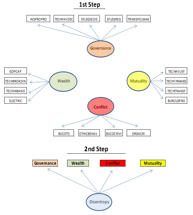
I am making a 2-steps approach to estimate a SEM model in the field of economics as depicted in the attached figure. In order to obtain the estimated values of the latent variables observation-by-observation for N=142 countries in the 1st step I am using the predict function of lavaan.
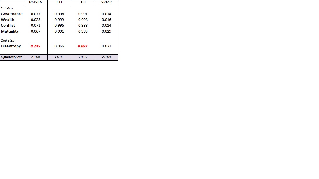
Whilst fit results for the individual measurement models of the 1st step are pretty good, at the moment I have not got acceptable RMSEA and TLI in the 2nd step (RMSEA: 0.245, TLI: 0.897) as shown in the following chart:
RMSEA CFI TLI SRMR
1st step
Governance 0.077 0.996 0.991 0.014
Wealth 0.028 0.999 0.998 0.016
Conflict 0.071 0.996 0.988 0.014
Mutuality 0.067 0.991 0.983 0.029
2nd step
Disentropy 0.245 0.966 0.897 0.023
Optimality cut < 0.08 > 0.95 > 0.95 < 0.08
I have a set of measurable variables for each of the four latent variables and am trying to improve the overall model following a trial-and-error method.
-
Could you give me some guidance on how to proceed in order to respecify the 2nd step model?
-
Will the 2nd step model improve if the individual 1st step models improve?
-
Could I perform any sort of statistical tests / analyses on all the available measurable variables in order to set the 1st step individual models determining an acceptable fit of the 2nd step model?
Thanks
(Note: this thread follows a post I submitted to this fórum - General SEM Discussions - on 04/25/2015)
[img_assist|nid=4093|title=2-step SEM Model|desc=|link=none|align=left|width=90|height=100]
Is there a reason why you're not doing this in a single step, as in my diagram attached to this post?
Edit: And do I understand correctly that your first step consists of fitting four separate, single-factor models, each to a different set of observable variables?
Rob's model presents all the data in one model, allowing the model to see, for instance, if the factors should be collapsed, or if items covary across factors plus much more: Far to be preferred!
With regard to the first question of why a 2-step model, my assumption was that by following the 1-step model option a good fit of the overall model could hide or compensate a poor fit of any of the underneath measurable models. Besides, I thought that the partition of the overall SEM model into a number of measurable models would facilitate the selection of the best observable variables to achieve a good fit.
Thus, in response to the second question, yes, the 1st step would consist on fitting four separate single-factor models each to a different set of observable variables.
Next an estimation of the values of the single factors (Governance, Wealth, Conflict and Mutuality) would be done, for instance using de lavPredict function. The 2nd step would consist on fitting the single factor model of Disentropy where the “measurable” variables would be the latent variables of the 1st step model for which we would have calculated values observation-by-observation. Obviously the two steps are related as the 2nd step is fed by the output of the 1st step. In the end, for my research I will need the “calculated values” of the 5 latent variables (G, W, C, M and D).
I attach a database including the values of 29 observable variables used in the model sorted by their correspondence to each of the four factors according to theoretical criteria. My aim is to select and fit the right observable variables to the four factors in order to achieve an acceptable goodness-of-fit of the overall model.
I will be grateful if you could give me your view about which way you think would be better to go: 1-step analysis versus 2-steps analysis, and some guidelines on how to proceed (apologies if the question is too broad or vague).
Thanks
I definitely recommend avoiding factor-score predictions as much as you can. You were on the right track in your previous post, where you described a model that included all the observable variables and all four latent variables. You could extend that model by adding Disentropy as an additional latent variable, underlying Wealth, Governance, Mutuality, and Conflict. If you need predictions on the five latent variables for additional analysis, they're relatively easy to get out of such a fitted model.
The problem there, of course, was that the model from your previous post did not fit the data very well. That could possibly be because some of the observable variables load substantially onto more than one factor, or because four factors are not enough, or because there's something else going on (bifactor structure?). Have you tried exploratory factor analysis? EFA might be an answer to your question #3 in your OP. I strongly suspect that some of the observable variables have substantial loadings on more than one factor. That would help explain why the fit indices are much better for each first-step single-factor analysis than they were for the model in your prior post.
If there are strong a priori theoretical or empirical reasons for grouping the variables together as they are in your spreadsheet, and you just want some kind of data-reduction in each of the four domains, you could consider something more straightforward, like taking the first principal component.
I have followed the proposed straightforward way; that’s to say, I have analyzed the first principal component. Definitely the output gets much better. I have got a number of alternative 1-step models that present a good fit.
For instance:
Model148 <- 'G =~ INSPROPRO + PRIMEDUC
W =~ GDPCAP + TECHINBAND
C =~ ETHICBEHAV + IRREPAY
M =~ TECHAVLAT + TECHFIRMABS + FOMASIZE
D =~ G + W +C + M'
fit148 <- sem(Model148, data = Datvarpap8)
summary(fit148, standardized = TRUE, fit.measures = TRUE, rsq = TRUE)
lavaan (0.5-20) converged normally after 46 iterations
Number of observations 142
Estimator ML
Minimum Function Test Statistic 31.397
Degrees of freedom 23
P-value (Chi-square) 0.113
Model test baseline model:
Minimum Function Test Statistic 1468.479
Degrees of freedom 36
P-value 0.000
User model versus baseline model:
Comparative Fit Index (CFI) 0.994
Tucker-Lewis Index (TLI) 0.991
Loglikelihood and Information Criteria:
Loglikelihood user model (H0) -1137.798
Loglikelihood unrestricted model (H1) -1122.100
Number of free parameters 22
Akaike (AIC) 2319.597
Bayesian (BIC) 2384.625
Sample-size adjusted Bayesian (BIC) 2315.016
Root Mean Square Error of Approximation:
RMSEA 0.051
90 Percent Confidence Interval 0.000 0.091
P-value RMSEA <= 0.05 0.453
Standardized Root Mean Square Residual:
SRMR 0.023
Thank you so much for your reasoning and indications, they have been very useful.
In prior posts you tell me that the prediction of the five latent variables would be easy to obtain from the fitted model. Could you please give me some guidelines and I will delve into them? Currently I am running the lavaan package in R-studio, but I am open to use any other software (preferably available on R or open source) with which I could complete the calculations.
I'm confused about what you did to select the observable variables to be entered into analysis. You mention both exploratory factor analysis and the first principal component, but EFA and PCA aren't the same thing.
Also, am I correct that this syntax,
produces a model in which G only has paths going to INSPROPRO and PRIMEDUC, W only has paths going to GDPCAP and TECHINBAND, C only has paths going to ETHICBEHAV and IRREPAY, and M only has paths going to TECHAVLAT, TECHFIRMABS, and FOMASIZE?
In my prior post I put EFA and PCA into the same bunch as they both pursue a reduction of factors, but you are right they are different things Actually, I meant PCA.
In order to select the variables I have used SPSS to run a principal components analysis (PCA) extracting only one component. The selection of observable variables of the model is based on an analysis of both the correlation and the covariance matrixes under the criteria that
The model exposed in the prior post presents a RMSEA of 0.051. I have tested other alternative models in compliance with the above criteria that even give lower RMSEAs.
As regards your second point, yes the syntax I have used produces the paths you state which correspond to the paths depicted in the graph that you posted on 01/24/2014.
I can run the lavPredict function of lavaan package to obtain the predicted values of the latent variables (Governance, Wealth, Conflict, Mutuality and Disentropy).
What other approaches can I follow in order to obtain predicted values of the latent variables?
Should I introduce new bidirectional relationships among the latent variables of Governance, Wealth, Conflict, Mutuality in order to assess covariance behavior, would that impact the obtained predicted values?
OK, I got it now.
What you're getting from lavaan is probably adequate. Does lavaan give you any idea of the quality of the factor-score predictions? It could be something like standard errors or prediction intervals, or some index of the degree of factor indeterminacy, like an R-squared or a Guttman's rho-star (which is the minimum possible correlation between two possible vectors of true factor scores).
These would represent covariance among those four factors that is NOT attributable to Disentropy, correct? I probably wouldn't do that. I'm not sure how many you could add and still keep the model identified.
I felt a bit uneasy when I noticed that three of the four lower-order factors in your model have nonzero loadings going to only two observable variables. Much of the time, one wants to have at least three observable indicators per common factor. I discussed it with some colleagues this morning, and we agreed that the model may not be identified, or possibly, that the model IS identified but its factor-score estimates are not.
I saved your Excel spreadsheet of data to a comma-separated .csv text file, and wrote an OpenMx script to fit your proposed model:
I ran it in OpenMx version 2.3.1.195, which is bleeding-edge, built from the source repository this morning. It's encouraging that I'm able to reproduce your chi-square statistic, RMSEA, CFI, and TLI. Also,
mxCheckIdentificationsays that the model is identified at the solution. However, it says that the model is locally unidentified at the start values, which makes me uneasy.My script predicts factor scores in three ways (see attachments): maximum-likelihood and weighted maximum-likelihood (which are built into OpenMx) and Thompson-Thurstone regression (which will be built into OpenMx in a future binary release). The ML predictions all have standard errors (also attached) that are either very large or
NA, which is troubling. Further, the three sets of predicted values do not agree that well (except concerning the higher-order factor, Disentropy)--in fact the regression and WML predictions for the lower-order factors correlate negatively!I can't say with certainty that there is a problem here, but I am concerned you don't have enough observable variables in the analysis to get good results out of your proposed model. Maybe reconsider your variable selection?
As far as I know, at the moment of writing this post Lavaan package does not provide standard errors or prediction intervals for factor score predictions (function lavpredict). It seems that a forthcoming version will do so.
I am glad to know that OpenMx version 2.3.1.195 does provide statistical information on score predictions. Your script and factor scores identification analysis answers my question regarding alternative software performing latent variables predicted values calculations. I am not an expert statistician but will put in the necessary time to learn how OpenMx version 2.3.1.195 works to run and check my next model simulations.
Evidently I need to formulate a model which is identified both at the solution and locally at the start values and factor score estimates. On the other hand, you are right I would like to have at least 3 observable variables per common factor. That should be so for improving the identification of the statistical model, but also to support better the theoretical framework of my research. In order to achieve it, I will elaborate more on EFA and PCA and include new observable variables if necessary.
Should I make any progress, I will post it, hopefully soon. Thanks
If you install OpenMx either from CRAN or by following these instructions (I recommend the latter), you'll get version 2.3.1, which is currently the official binary release. If you really want to build from the current source repository, instructions are here, but that's probably not necessary. However, you'd get built-in regression factor-scoring for RAM models if you build from source.
I am running your proposed script on OpenMx versión 2.3.1 (binary release). I have tested alternative models that reconsider the observable variables selection and increase the number of them per common factor . However they all present similar outputs and models are locally identified at solution but not locally identified at the start values. Statistics Chisquare, RMSEA, CFI, TLI look well.
With regard to the predicted factor score values that you posted in the blog, I don’t understand why your values differ so much from the ones I have obtained. The attached word document shows the details of the test I have ran where the statistics (Chisq, RMSEA,…) match with yours but the predicted values are so different!
Besides, I haven’t been able to obtain the Thompson-Thurstone regression coefficients. I assume this is because I am not using the repository OpenMx version, right? Would that explain as well why the rest of my predicted values (ml and wml) do not match with yours?
In fact, the TT regression coefficients seem to be the predicted factor scores that - from a theoretical standpoint – make the best sense for my research, and I would like to be able to obtain them by myself in order to conduct further analyses.
Would the use of the repository versión sort out the issues I've got with predicted factor scores values ?
Thanks on advance
OK, then maybe identification isn't a problem.
Concerning the discrepancy between the score estimates in my post and the score estimates you're getting, I suspect it has everything to do with the package version. The build of OpenMx I was using likely contained several changes related to
mxFactorScores()since version 2.3.1. These changes were included in the subsequent binary release, version 2.5.2 (release date 2/23/16):Note in particular the second bullet point. I suspect you and I are getting the same factor scores, but in a different order.
You could build from the source repository if you really want to, but updating to OpenMx version 2.5.2, either from CRAN or from our own virginia.edu repository, should suffice for your purposes.
In OpenMx version 2.5.2, you can get the Thompson-Thurstone regression score estimates straight from
mxFactorScores()(see first bullet point above). I notice in your MS Word document that you got the error "system is computationally singular" when you tried to manually calculate the TT regression estimates. In cases like that--where a matrix is positive-definite but nearly singular--you can often still obtain an its inverse if you replacesolve(myMatrix)withchol2inv(chol(myMatrix)). I'm mentioning this for the sake of other users who search this website for that error message. Also, this trick won't work if the matrix is exactly singular.