Examples, Path Specification¶

Regression, Path Specification¶

Our next example will show how regression can be carried out from a path-centric structural modeling perspective. This example is in three parts; a simple regression, a multiple regression, and multivariate regression. There are two versions of each example are available; one with raw data, and one where the data is supplied as a covariance matrix and vector of means. These examples are available in the following files:

SimpleRegression_PathCov.R
SimpleRegression_PathRaw.R
MultipleRegression_PathCov.R
MultipleRegression_PathRaw.R
MultivariateRegression_PathCov.R
MultivariateRegression_PathRaw.R

A parallel version of this example, using matrix specification of models rather than paths, can be found here link.

Simple Regression¶

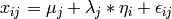
We begin with a single dependent variable (y) and a single independent variable (x). The relationship between these variables takes the following form:

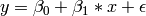
$\begin{eqnarray*} y = \beta_{0} + \beta_{1} * x + \epsilon \end{eqnarray*}$

In this model, the mean of y is dependent on both regression coefficients (and by extension, the mean of x). The variance of y depends on both the residual variance and the product of the regression slope and the variance of x. This model contains five parameters from a structural modeling perspective $\beta_{0}$ , $\beta_{1}$ , $\sigma^{2}_{\epsilon}$ , and the mean and variance of x). We are modeling a covariance matrix with three degrees of freedom (two variances and one variance) and a means vector with two degrees of freedom (two means). Because the model has as many parameters (5) as the data have degrees of freedom, this model is fully saturated.

Data¶

Our first step to running this model is to put include the data to be analyzed. The data must first be placed in a variable or object. For raw data, this can be done with the read.table function. The data provided has a header row, indicating the names of the variables.

myRegDataRaw <- read.table("myRegData.txt",header=TRUE)

The names fo the variables provided by the header row can be displayed with the names() function.

> names(myRegDataRaw)
[1] "w" "x" "y" "z"

As you can see, our data has four variables in it. However, our model only contains two variables, x and y. To use only them, we’ll select only the variables we want and place them back into our data object. That can be done with the R code below.

SimpleDataRaw <- myRegDataRaw[,c("x","y")]

For covariance data, we do something very similar. We create an object to house our data. Instead of reading in raw data from an external file, we can also include a covariance matrix. This requires the matrix() function, which needs to know what values are in the covariance matrix, how big it is, and what the row and column names are. As our model also references means, we’ll include a vector of means in a separate object. Data is selected in the same way as before.

myRegDataCov <- matrix(
    c(0.808,-0.110, 0.089, 0.361,
     -0.110, 1.116, 0.539, 0.289,
      0.089, 0.539, 0.933, 0.312,
      0.361, 0.289, 0.312, 0.836),
    nrow=4,
    dimnames=list(
        c("w","x","y","z"),
        c("w","x","y","z"))
)

SimpleDataCov <- myRegDataCov[c("x","y"),c("x","y")]

myRegDataMeans <- c(2.582, 0.054, 2.574, 4.061)

SimpleDataMeans <- myRegDataMeans[c(2,3)]

Model Specification¶

The following code contains all of the components of our model. Before running a model, the OpenMx library must be loaded into R using either the require() or library() function. All objects required for estimation (data, paths, and a model type) are included in their own arguments or functions. This code uses the mxModel function to create an MxModel object, which we’ll then run.

require(OpenMx)
uniRegModel <- mxModel("Simple Regression -- Path Specification",
    type="RAM",
    mxData(
        observed=SimpleDataRaw,
        type="raw"
    ),
    manifestVars=c("x", "y"),
    # variance paths
    mxPath(
        from=c("x", "y"),
        arrows=2,
        free=TRUE,
        values = c(1, 1),
        labels=c("varx", "residual")
    ),
    # regression weights
    mxPath(
        from="x",
        to="y",
        arrows=1,
        free=TRUE,
        values=1,
        labels="beta1"
    ),
    # means and intercepts
    mxPath(
        from="one",
        to=c("x", "y"),
        arrows=1,
        free=TRUE,
        values=c(1, 1),
        labels=c("meanx", "beta0")
    )
) # close model

This mxModel function can be split into several parts. First, we give the model a title. The first argument in an mxModel function has a special function. If an object or variable containing an MxModel object is placed here, then mxModel adds to or removes pieces from that model. If a character string (as indicated by double quotes) is placed first, then that becomes the name of the model. Models may also be named by including a name argument. This model is named Simple Regression -- Path Specification.

The next part of our code is the type` argument. By setting type="RAM", we tell OpenMx that we are specifying a RAM model for covariances and means, and that we are doing so using the mxPath function. With this setting, OpenMx uses the specified paths to define the expected covariance and means of our data.

The third component of our code creates an MxData object. The example above, reproduced here, first references the object where our data is, then uses the type argument to specify that this is raw data.

mxData(
    observed=SimpleDataRaw,
    type="raw"
)

If we were to use a covariance matrix and vector of means as data, we would replace the existing mxData function with this one:

mxData(
    observed=SimpleDataCov,
    type="cov",
    numObs=100,
    means=SimpleRegMeans
)

We must also specify the list of observed variables using the manifestVars argument. In the code below, we include a list of both observed variables, x and y.

The last features of our code are three mxPath functions, which describe the relationships between variables. Each function first describes the variables involved in any path. Paths go from the variables listed in the from argument, and to the variables listed in the to argument. When arrows is set to 1, then one-headed arrows (regressions) are drawn from the from variables to the to variables. When arrows is set to 2, two headed arrows (variances or covariances) are drawn from the the from variables to the to variables. If arrows is set to 2, then the to argument may be omitted to draw paths both to and from the list of from` variables.

The variance terms of our model (that is, the variance of x and the residual variance of y) are created with the following mxPath function. We want two headed arrows from x to x, and from y to y. These paths should be freely estimated (free=TRUE), have starting values of 1, and be labeled "varx" and "residual", respectively.

mxPath(
    from=c("x", "y"),
    arrows=2,
    free=TRUE,
    values = c(1, 1),
    labels=c("varx", "residual")
)

The regression term of our model (that is, the regression of y on x) is created with the following mxPath function. We want a single one-headed arrow from x to y. This path should be freely estimated (free=TRUE), have a starting value of 1, and be labeled "beta1".

mxPath(
        from="x",
        to="y",
        arrows=1,
        free=TRUE,
        values=1,
        labels="beta1"
    )

We also need means and intercepts in our model. Exogenous or independent variables have means, while endogenous or dependent variables have intercepts. These can be included by regressing both x and y on a constant, which can be refered to in OpenMx by "one". The intercept terms of our model are created with the following mxPath function. We want single one-headed arrows from the constant to both x and y. These paths should be freely estimated (free=TRUE), have a starting value of 1, and be labeled meanx and "beta1", respectively.

mxPath(
    from="one",
    to=c("x", "y"),
    arrows=1,
    free=TRUE,
    values=c(1, 1),
    labels=c("meanx", "beta0")
)

Our model is now complete!

Model Fitting¶

We’ve created an MxModel object, and placed it into an object or variable named uniRegModel. We can run this model by using the mxRun function, which is placed in the object uniRegFit in the code below. We then view the output by referencing the output slot, as shown here.

uniRegFit <- mxRun(uniRegModel)

uniRegFit@output

The output slot contains a great deal of information, including parameter estimates and information about the matrix operations underlying our model. A more parsimonious report on the results of our model can be viewed using the summary function, as shown here.

summary(uniRegFit)

Multiple Regression¶

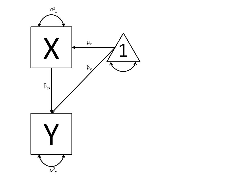
In the next part of this demonstration, we move to multiple regression. The regression equation for our model looks like this:

$\begin{eqnarray*} y = \beta_{0} + \beta_{x} * x + \beta_{z} * z + \epsilon \end{eqnarray*}$

Our dependent variable y is now predicted from two independent variables, x and z. Our model includes 3 regression parameters ( $\beta_{0}$ , $\beta_{x}$ , $\beta_{z}$ ), a residual variance (:math:`sigma^{2}_{epsilon}) and the observed means, variances and covariance of x and z, for a total of 9 parameters. Just as with our simple regression, this model is fully saturated.

We prepare our data the same way as before, selecting three variables instead of two.

MultipleDataRaw <- myRegDataRaw[,c("x","y","z")]

MultipleDataCov <- myRegDataCov[c("x","y","z"),c("x","y","z")]

MultipleDataMeans <- myRegDataMeans[c(2,3,4)]

Now, we can move on to our code. It is identical in structure to our simple regression code, but contains additional paths for the new parts of our model.

require(OpenMx)
multiRegModel <- mxModel("Multiple Regression -- Path Specification",
    type="RAM",
    mxData(
        observed=MultipleDataRaw,
        type="raw"
    ),
    manifestVars=c("x", "y", "z"),
    # variance paths
    mxPath(
        from=c("x", "y", "z"),
        arrows=2,
        free=TRUE,
        values = c(1, 1, 1),
        labels=c("varx", "residual", "varz")
    ),
    # covariance of x and z
    mxPath(
        from="x",
        to="y",
        arrows=2,
        free=TRUE,
        values=0.5,
        labels="covxz"
    ),
    # regression weights
    mxPath(
        from=c("x","z"),
        to="y",
        arrows=1,
        free=TRUE,
        values=1,
        labels=c("betax","betaz")
    ),
    # means and intercepts
    mxPath(
        from="one",
        to=c("x", "y", "z"),
        arrows=1,
        free=TRUE,
        values=c(1, 1),
        labels=c("meanx", "beta0", "meanz")
    )
) # close model

multiRegFit <- mxRun(multiRegModel)

multiRegFit@output

summary(multiRegFit)

The first bit of our code should look very familiar. require(OpenMx) makes sure the OpenMx library is loaded into R. This only needs to be done at the first model of any R session. The type="RAM" argument is identical. The mxData function references our multiple regression data, which contains one more variable than our simple regression data. Similarly, our manifestVars list contains an extra label, "z".

The mxPath functions work just as before. Our first function defines the variances of our variables. Whereas our simple regression included just the variance of x and the residual variance of y, our multiple regression includes the variance of z as well.

Our second mxPath function specifies a two-headed arrow (covariance) between x and z. We’ve omitted the to argument from two-headed arrows up until now, as we have only required variaces. Covariances may be specified by using both the from and to arguments. This path is freely estimated, has a starting value of 0.5, and is labeled "covxz.

mxPath(
    from="x",
    to="y",
    arrows=2,
    free=TRUE,
    values=0.5,
    labels="covxz"
),

The third and fourth mxPath functions mirror the second and third mxPath functions from our simple regression, defining the regressions of y on both x and z as well as the means and intercepts of our model.

The model is run and output is viewed just as before, using the mxRun function, @output and the summary function to run, view and summarize the completed model.

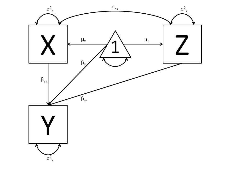
Multivariate Regression¶

The structural modeling approach allows for the inclusion of not only multiple independent variables (i.e., multiple regression), but multiple dependent variables as well (i.e., multivariate regression). Versions of multivariate regression are sometimes fit under the heading of path analysis. This model will extend the simple and multiple regression frameworks we’ve discussed above, adding a second dependent variable “w”.

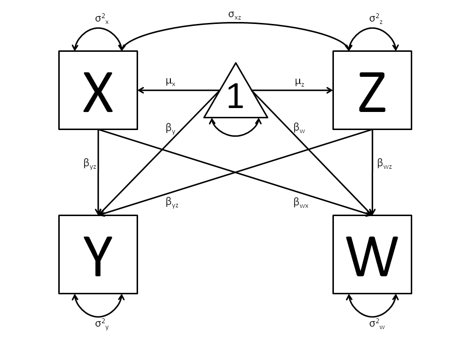
$\begin{eqnarray*} y = \beta_{y} + \beta_{yx} * x + \beta_{yz} * z\epsilon\\ w = \beta_{w} + \beta_{wx} * x + \beta_{wz} * z\epsilon \end{eqnarray*}$

We now have twice as many regression parameters, a second residual variance, and the same means, variances and covariances of our independent variables. As with all of our other examples, this is a fully saturated model.

Data import for this analysis will actually be slightly simpler than before. The data we imported for the previous examples contains only the four variables we need for this model. We can use myRegDataRaw, myRegDataCov, and``myRegDataMeans`` in our models.

myRegDataRaw<-read.table("myRegData.txt",header=TRUE)

myRegDataCov <- matrix(
    c(0.808,-0.110, 0.089, 0.361,
     -0.110, 1.116, 0.539, 0.289,
      0.089, 0.539, 0.933, 0.312,
      0.361, 0.289, 0.312, 0.836),
    nrow=4,
    dimnames=list(
        c("w","x","y","z"),
        c("w","x","y","z"))
)

myRegDataMeans <- c(2.582, 0.054, 2.574, 4.061)

Our code should look very similar to our previous two models. It includes the same type argument, mxData function, and manifestVars argument as previous models, with a different version of the data and additional variables in the latter two components.

multivariateRegModel <- mxModel("MultiVariate Regression -- Path Specification",
    type="RAM",
    mxData(
        observed=myRegDataRaw,
        type="raw"
    ),
    manifestVars=c("w", "x", "y", "z"),
    # variance paths
    mxPath(
        from=c("w", "x", "y", "z"),
        arrows=2,
        free=TRUE,
        values = c(1, 1, 1),
        labels=c("residualw", "varx", "residualy", "varz")
    ),
    # covariance of x and z
    mxPath(
        from="x",
        to="y",
        arrows=2,
        free=TRUE,
        values=0.5,
        labels="covxz"
    ),
    # regression weights for y
    mxPath(
        from=c("x","z"),
        to="y",
        arrows=1,
        free=TRUE,
        values=1,
        labels=c("betayx","betayz")
    ),
    # regression weights for w
    mxPath(
        from=c("x","z"),
        to="w",
        arrows=1,
        free=TRUE,
        values=1,
        labels=c("betawx","betawz")
    ),
    # means and intercepts
    mxPath(
        from="one",
        to=c("w", "x", "y", "z"),
        arrows=1,
        free=TRUE,
        values=c(1, 1),
        labels=c("betaw", "meanx", "betay", "meanz")
    )
) # close model

multivariateRegFit <- mxRun(multivariateRegModel)

multivariateRegFit@output

summary(multivariateRegFit)

The only additional components to our mxPath functions are the inclusion of the “w” variable and the additional set of regression coefficients for “w”. Running the model and viewing output works exactly as before.

These models may also be specified using matrices instead of paths. See link for matrix specification of these models.

Factor Analysis, Path Specification¶

This example will demonstrate latent variable modeling via the common factor model using path-centric model specification. We’ll walk through two applications of this approach: one with a single latent variable, and one with two latent variables. As with previous examples, these two applications are split into four files, with each application represented separately with raw and covariance data. These examples can be found in the following files:

OneFactorModel_PathCov.R
OneFactorModel_PathRaw.R
TwoFactorModel_PathCov.R
TwoFactorModel_PathRaw.R

A parallel version of this example, using matrix specification of models rather than paths, can be found here link.

Common Factor Model¶

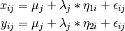
The common factor model is a method for modeling the relationships between observed variables believed to measure or indicate the same latent variable. While there are a number of exploratory approaches to extracting latent factor(s), this example uses structural modeling to fit confirmatory factor models. The model for any person and path diagram of the common factor model for a set of variables :math:`x_{1}’-:math:`x_{6}’ are given below.

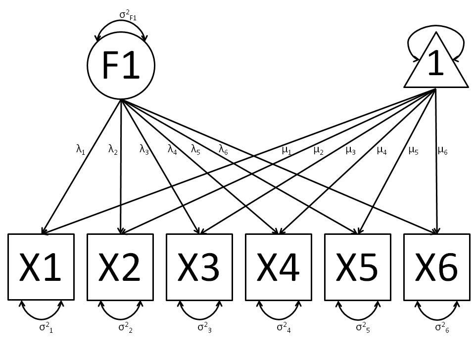
$\begin{eqnarray*} x_{ij} = \mu_{j} + \lambda_{j} * \eta_{i} + \epsilon_{ij} \end{eqnarray*}$

While 19 parameters are displayed in the equation and path diagram above (6 manifest variances, six manifest means, six factor loadings and one factor variance), we must constrain either the factor variance or one factor loading to a constant to identify the model and scale the latent variable. As such, this model contains 18 parameters. Unlike the manifest variable examples we’ve run up until now, this model is not fully saturated. The means and covariance matrix for six observed variables contain 27 degrees of freedom, and thus our model contains 9 degrees of freedom.

Data¶

Our first step to running this model is to put include the data to be analyzed. The data for this example contain nine variables. We’ll select the six we want for this model using the selection operators used in previous examples. Both raw and covariance data are included below, but only one is required for any model.

myFADataRaw <- read.table("myFAData.txt",header=TRUE)

> names(myFADataRaw)
[1] "x1" "x2" "x3" "x4" "x5" "x6" "y1" "y2" "y3"

oneFactorRaw <- myFADataRaw[,c("x1", "x2", "x3", "x4", "x5", "x6")]

myFADataCov <- matrix(
    c(0.997, 0.642, 0.611, 0.672, 0.637, 0.677, 0.342, 0.299, 0.337,
      0.642, 1.025, 0.608, 0.668, 0.643, 0.676, 0.273, 0.282, 0.287,
      0.611, 0.608, 0.984, 0.633, 0.657, 0.626, 0.286, 0.287, 0.264,
      0.672, 0.668, 0.633, 1.003, 0.676, 0.665, 0.330, 0.290, 0.274,
      0.637, 0.643, 0.657, 0.676, 1.028, 0.654, 0.328, 0.317, 0.331,
      0.677, 0.676, 0.626, 0.665, 0.654, 1.020, 0.323, 0.341, 0.349,
      0.342, 0.273, 0.286, 0.330, 0.328, 0.323, 0.993, 0.472, 0.467,
      0.299, 0.282, 0.287, 0.290, 0.317, 0.341, 0.472, 0.978, 0.507,
      0.337, 0.287, 0.264, 0.274, 0.331, 0.349, 0.467, 0.507, 1.059),
    nrow=9,
    dimnames=list(
        c("x1", "x2", "x3", "x4", "x5", "x6", "y1", "y2", "y3"),
        c("x1", "x2", "x3", "x4", "x5", "x6", "y1", "y2", "y3")),
    )

oneFactorCov <- myFADataCov[c("x1", "x2", "x3", "x4", "x5", "x6"),c("x1", "x2", "x3", "x4", "x5", "x6")]

myFADataMeans <- c(2.988, 3.011, 2.986, 3.053, 3.016, 3.010, 2.955, 2.956, 2.967)

oneFactorMeans <- myFADataMeans[1:6]

Model Specification¶

Creating a path-centric factor model will use many of the same functions and arguments used in previous path-centric examples. However, the inclusion of latent variables adds a few extra pieces to our model. Before running a model, the OpenMx library must be loaded into R using either the require() or library() function. All objects required for estimation (data, paths, and a model type) are included in their own arguments or functions. This code uses the mxModel function to create an MxModel object, which we’ll then run.

require(OpenMx)

oneFactorModel<-mxModel("Common Factor Model - Path",
    type="RAM",
    mxData(
        observed=oneFactorRaw,
        type="raw"),
    manifestVars=c("x1","x2","x3","x4","x5","x6"),
    latentVars="F1",
    # residual variances
    mxPath(from=c("x1","x2","x3","x4","x5","x6"),
        arrows=2,
        free=TRUE,
        values=c(1,1,1,1,1,1),
        labels=c("e1","e2","e3","e4","e5","e6")
        ),
    # latent variance
    mxPath(from="F1",
        arrows=2,
        free=TRUE,
        values=1,
        labels ="varF1"
        ),
    # factor loadings
    mxPath(from="F1",
        to=c("x1","x2","x3","x4","x5","x6"),
        arrows=1,
        free=c(FALSE,TRUE,TRUE,TRUE,TRUE,TRUE),
        values=c(1,1,1,1,1,1),
        labels =c("l1","l2","l3","l4","l5","l6")
        ),
    # means
    mxPath(from="one",
        to=c("x1","x2","x3","x4","x5","x6","F1"),
        arrows=1,
        free=c(TRUE,TRUE,TRUE,TRUE,TRUE,TRUE,FALSE),
        values=c(1,1,1,1,1,1,0),
        labels =c("meanx1","meanx2","meanx3",
            "meanx4","meanx5","meanx6",
            NA)
        )
    ) # close model

As with previous examples, this model begins with a name for the model and a type="RAM" argument. The name for the model may be omitted, or may be specified an any other place in the model using the name argument. Including type="RAM" allows the mxModel function to interpret the mxPath functions that follow and turn those paths into an expected covariance matrix and means vector for the ensuing data. The mxData function works just as in previous examples, and the raw data specification included in the code:

mxData(
    observed=oneFactorRaw,
    type="raw")

can be replaced with a covariance matrix and means, like so:

oneFactorModel<-mxModel("Common Factor Model - Path",
    type="RAM",
    mxData(
        observed=oneFactorCov,
        type="cov",
        numObs=500,
        means=oneFactorMeans)

The first departure from our previous examples can be found in the addition of the latentVars argument after the manifestVars argument. The manifestVars argument includes the six variables in our observed data. The latentVars argument provides a name for the latent variable, so that it may be referenced in mxPath functions.

manifestVars=c("x1","x2","x3","x4","x5","x6"),
latentVars="F1"

Our model is defined by four mxPath functions. The first defines the residual variance terms for our six observed variables. The to argument is not required, as we are specifiying two headed arrows both from and to the same variables, as specified in the from argument. These six variances are all freely estimated, have starting values of 1, and are labeled e1 through e6.

mxPath(from=c("x1","x2","x3","x4","x5","x6"),
    arrows=2,
    free=TRUE,
    values=c(1,1,1,1,1,1),
    labels=c("e1","e2","e3","e4","e5","e6")
)

We also must specify the variance of our latent variable. This code is identical to our residual variance code above, with the latent variable "F1" replacing our six manifest variables.

mxPath(from="F1",
    arrows=2,
    free=TRUE,
    values=1,
    labels ="varF1"
)

Next come the factor loadings. These are specified as assymetric paths (regressions) of the manifest variables on the latent variable "F1". As we have to scale the latent variable, the first factor loading has been given a fixed value of one by setting the first elements of the free and values arguments to FALSE and 1, respectively. Alternatively, the latent variable could have been scaled by fixing the factor variance to 1 in the previous mxPath function and freely estimating all factor loadings. The five factor loadings that are freely estimated are all given starting values of 1 and labels l2 through l6.

mxPath(from="F1",
    to=c("x1","x2","x3","x4","x5","x6"),
    arrows=1,
    free=c(FALSE,TRUE,TRUE,TRUE,TRUE,TRUE),
    values=c(1,1,1,1,1,1),
    labels =c("l1","l2","l3","l4","l5","l6")
)

Lastly, we must specify the mean structure for this model. As there are a total of seven variables in this model (six manifest and one latent), we have the potential for seven means. However, we must constrain at least one mean to a constant value, as there is not sufficient information to yield seven mean and intercept estimates from the six observed means. The six observed variables receive freely estimated intercepts, while the factor mean is fixed to a value of zero in the code below.

mxPath(from="one",
    to=c("x1","x2","x3","x4","x5","x6","F1"),
    arrows=1,
    free=c(TRUE,TRUE,TRUE,TRUE,TRUE,TRUE,FALSE),
    values=c(1,1,1,1,1,1,0),
    labels =c("meanx1","meanx2","meanx3",
        "meanx4","meanx5","meanx6",
        NA)
)

The model can now be run using the mxRun function, and the output of the model can be accessed from the output slot of the resulting model. A summary of the output can be reached using summary().

oneFactorFit <- mxRun(oneFactorModel)

oneFactorFit@output

summary(oneFactorFit)

Two Factor Model¶

The common factor model can be extended to include multiple latent variables. The model for any person and path diagram of the common factor model for a set of variables $x_{1}'-:math:`x_{3}$ and $y_{1}'-:math:`y_{3}$ are given below.

$\begin{eqnarray*} x_{ij} = \mu_{j} + \lambda_{j} * \eta_{1i} + \epsilon_{ij}\\ y_{ij} = \mu_{j} + \lambda_{j} * \eta_{2i} + \epsilon_{ij} \end{eqnarray*}$

Our model contains 21 parameters (6 manifest variances, six manifest means, six factor loadings, two factor variances and one factor covariance), but each factor requires one identification constraint. Like in the common factor model above, we’ll constrain one factor loading for each factor to a value of one. As such, this model contains 19 parameters. The means and covariance matrix for six observed variables contain 27 degrees of freedom, and thus our model contains 8 degrees of freedom.

The data for the two factor model can be found in the myFAData files introduced in the common factor model. For this model, we’ll select three x variables (x1-x3) and three y variables (y1-y3`).

twoFactorRaw <- myFADataRaw[,c("x1", "x2", "x3", "y1", "y2", "y3")]

twoFactorCov <- myFADataCov[c("x1", "x2", "x3", "y1", "y2", "y3"),c("x1", "x2", "x3", "y1", "y2", "y3")]

twoFactorMeans <- myFADataMeans[c(1:3,7:9)]

Specifying the two factor model is virtually identical to the single factor case. The last three variables of our manifestVars argument have changed from "x4","x5","x6" to “y1”,”y2”,”y3”, which is carried through references to the variables in later mxPath functions.

twofactorModel<-mxModel("Two Factor Model - Path",
    type="RAM",
    mxData(
        observed=twoFactorRaw,
        type="raw"
        ),
    manifestVars=c("x1","x2","x3","y1","y2","y3"),
    latentVars=c("F1","F2"),
    # residual variances
    mxPath(from=c("x1","x2","x3","y1","y2","y3"),
        arrows=2,
        free=TRUE,
        values=c(1,1,1,1,1,1),
        labels=c("e1","e2","e3","e4","e5","e6")
        ),
    # latent variances and covariance
    mxPath(from=c("F1","F2"),
        arrows=2,
        all=2,
        free=TRUE,
        values=c(1, .5,
                .5, 1),
        labels=c("varF1","cov","cov","varF2")
        ),
    # factor loadings for x variables
    mxPath(from="F1",
        to=c("x1","x2","x3"),
        arrows=1,
        free=c(FALSE,TRUE,TRUE),
        values=c(1,1,1),
        labels=c("l1","l2","l3")
        ),
    #factor loadings for y variables
    mxPath(from="F2",
        to=c("y1","y2","y3"),
        arrows=1,
        free=c(FALSE,TRUE,TRUE),
        values=c(1,1,1),
        labels=c("l4","l5","l6")
        ),
    #means
    mxPath(from="one",
        to=c("x1","x2","x3","y1","y2","y3","F1","F2"),
        arrows=1,
        free=c(TRUE,TRUE,TRUE,TRUE,TRUE,TRUE,FALSE,FALSE),
        values=c(1,1,1,1,1,1,0,0),
        labels=c("meanx1","meanx2","meanx3",
                 "meany1","meany2","meany3",
                  NA,NA)
    )
)

We’ve covered the type argument, mxData function and manifestVars and latentVars arguments previously, so now we’ll focus on the changes this model makes to the mxPath functions. The first and last mxPath functions, which detail residual variances and intercepts, accomodate the changes in manifest and latent variables but carry out identical functions to the common factor model.

# residual variances
mxPath(from=c("x1","x2","x3","y1","y2","y3"),
    arrows=2,
    free=TRUE,
    values=c(1,1,1,1,1,1),
    labels=c("e1","e2","e3","e4","e5","e6")
    ),
#means
mxPath(from="one",
    to=c("x1","x2","x3","y1","y2","y3","F1","F2"),
    arrows=1,
    free=c(TRUE,TRUE,TRUE,TRUE,TRUE,TRUE,FALSE,FALSE),
    values=c(1,1,1,1,1,1,0,0),
    labels=c("meanx1", "meanx2", "meanx3", "meany1","meany2","meany3",
                  NA,NA)
)

The second, third and fourth mxPath functions provide some changes to the model. The second mxPath function specifies the variances and covariance of the two latent variables. Like previous examples, we’ve omitted the to argument for this set of two-headed paths. Unlike previous examples, we’ve set the all argument to TRUE, which creates all possible paths between the variables. As omitting the to argument is identical to putting identical variables in the from and to arguments, we are creating all possible paths from and to our two latent variables. This results in four paths: from F1 to F2 (the variance of F1), from F1 to F2 (the covariance of the latent variables), from F2 to F1 (again, the covariance), and from F2 to F2 (the variance of F2). As the covariance is both the second and third path on this list, the second and third elements of both the values argument (.5) and the labels argument ("cov") are the same.

mxPath(from=c("F1","F2"),
    arrows=2,
    all=2,
    free=TRUE,
    values=c(1, .5,
            .5, 1),
    labels=c("varF1","cov","cov","varF2")
)

The third and fourth mxPath functions define the factor loadings for each of the latent variables. We’ve split these loadings into two functions, one for each latent variable. The first loading for each latent variable is fixed to a value of one, just as in the previous example.

# factor loadings for x variables
mxPath(from="F1",
    to=c("x1","x2","x3"),
    arrows=1,
    free=c(FALSE,TRUE,TRUE),
    values=c(1,1,1),
    labels=c("l1","l2","l3")
)
#factor loadings for y variables
mxPath(from="F2",
    to=c("y1","y2","y3"),
    arrows=1,
    free=c(FALSE,TRUE,TRUE),
    values=c(1,1,1),
    labels=c("l4","l5","l6")
)

The model can now be run using the mxRun function, and the output of the model can be accessed from the output slot of the resulting model. A summary of the output can be reached using summary().

oneFactorFit <- mxRun(oneFactorModel)

oneFactorFit@output

summary(oneFactorFit)

These models may also be specified using matrices instead of paths. See link for matrix specification of these models.

Time Series, Path Specification¶

This example will demonstrate a growth curve model using path-centric specification. As with previous examples, this application is split into two files, one each raw and covariance data. These examples can be found in the following files:

LGC_PathCov.R
LGC_PathRaw.R

A parallel version of this example, using matrix-centric specification of models rather than paths, can be found here link.

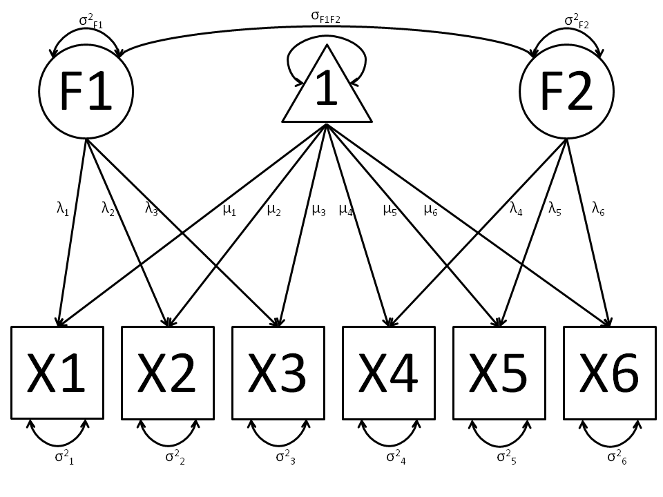
Latent Growth Curve Model¶

The latent growth curve model is a variation of the factor model for repeated measurements. For a set of manifest variables $x_{i1}$ - $x_{i5}$ measured at five discrete times for people indexed by the letter i, the growth curve model can be expressed both algebraically and via a path diagram as shown here:

. math::

nowrap:

begin{eqnarray*} x_{ij} = Intercept_{i} + lambda_{j} * Slope_{i} + epsilon_{i} end{eqnarray*}

The values and specification of the $\lambda$ parameters allow for alterations to the growth curve model. This example will utilize a linear growth curve model, so we will specify $\lambda$ to increase linearly with time. If the observations occur at regular intervals in time, then $\lambda$ can be specified with any values increasing at a constant rate. For this example, we’ll use [0, 1, 2, 3, 4] so that the intercept represents scores at the first measurement occasion, and the slope represents the rate of change per measurement occasion. Any linear transformation of these values can be used for linear growth curve models.

Our model for any number of variables contains 6 free parameters; two factor means, two factor variances, a factor covariance and a (constant) residual variance for the manifest variables. Our data contains five manifest variables, and so the covariance matrix and means vector contain 20 degrees of freedom. Thus, the linear growth curve model fit to these data has 14 degrees of freedom.

Data¶

The first step to running our model is to import data. The code below is used to import both raw data and a covariance matrix and means vector, either of which can be used for our growth curve model. This data contains five variables, which are repeated measurements of the same variable "x". As growth curve models make specific hypotheses about the variances of the manifest variables, correlation matrices generally aren’t used as data for this model.

myLongitudinalData <- read.table("myLongitudinalData.txt",header=T)

myLongitudinalDataCov<-matrix(
          c(6.362, 4.344, 4.915,  5.045,  5.966,
            4.344, 7.241, 5.825,  6.181,  7.252,
            4.915, 5.825, 9.348,  7.727,  8.968,
            5.045, 6.181, 7.727, 10.821, 10.135,
            5.966, 7.252, 8.968, 10.135, 14.220),
          nrow=5,
          dimnames=list(
                   c("x1","x2","x3","x4","x5"),
       c("x1","x2","x3","x4","x5"))
      )

myLongitudinalDataMean <- c(9.864, 11.812, 13.612, 15.317, 17.178)

Model Specification¶

We’ll create a path-centric factor model with the same functions and arguments used in previous path-centric examples. This model is a special type of two-factor model, with fixed factor loadings, constant residual variance and manifest means dependent on latent means.

Before running a model, the OpenMx library must be loaded into R using either the require() or library() function. This code uses the mxModel function to create an MxModel object, which we’ll then run.

require(OpenMx)

growthCurveModel <- mxModel("Linear Growth Curve Model, Path Specification",
    type="RAM",
    mxData(myLongitudinalData,
        type="raw"),
    manifestVars=c("x1","x2","x3","x4","x5"),
    latentVars=c("intercept","slope"),
    # residual variances
    mxPath(from=c("x1","x2","x3","x4","x5"),
        arrows=2,
        free=TRUE,
        values = c(1, 1, 1, 1, 1),
        labels=c("residual","residual","residual","residual","residual")
    ),
    # latent variances and covariance
    mxPath(from=c("intercept","slope"),
        arrows=2,
        all=TRUE,
        free=TRUE,
        values=c(1, 1, 1, 1),
        labels=c("vari", "cov", "cov", "vars")
    ),
    # intercept loadings
    mxPath(from="intercept",
        to=c("x1","x2","x3","x4","x5"),
        arrows=1,
        free=FALSE,
        values=c(1, 1, 1, 1, 1)
    ),
    # slope loadings
    mxPath(from="slope",
        to=c("x1","x2","x3","x4","x5"),
        arrows=1,
        free=FALSE,
        values=c(0, 1, 2, 3, 4
    ),
    # manifest means
    mxPath(from="one",
        to=c("x1", "x2", "x3", "x4", "x5"),
        arrows=1,
        free=FALSE,
        values=c(0, 0, 0, 0, 0)),
    # latent means
    mxPath(from="one",
        to=c("intercept", "slope"),
        arrows=1,
        free=TRUE,
        values=c(1, 1),
        labels=c("meani", "means")
    )
) # close model

The model begins with a name, in this case “Linear Growth Curve Model, Path Specification”. If the first argument is an object containing an MxModel object, then the model created by the mxModel function will contain all of the named entites in the referenced model object. The type="RAM" argument specifies a RAM model, allowing the mxModel to define an expected covariance matrix from the paths we supply.

Data is supplied with the mxData function. This example uses raw data, but the mxData function in the code above could be replaced with the function below to include covariance data.

mxData(myLongitudinalDataCov,
    type="cov",
    numObs=500,
    means=myLongitudinalDataMeans)

Next, the manifest and latent variables are specified with the manifestVars and latentVars arguments. The two latent variables in this model are named "Intercept" and "Slope".

There are six mxPath functions in this model. The first two specify the variances of the manifest and latent variables, respectively. The manifest variables are specified below, which take the form of residual variances. The to argument is omitted, as it is not required to specify two-headed arrows. The residual variances are freely estimated, but held to a constant value across the five measurement occasions by giving all five variances the same label.

# residual variances
mxPath(from=c("x1","x2","x3","x4","x5"),
    arrows=2,
    free=TRUE,
    values = c(1, 1, 1, 1, 1),
    labels=c("residual","residual","residual","residual","residual")
)

Next are the variances and covariance of the two latent variables. Like the last function, we’ve omitted the to argument for this set of two-headed paths. However, we’ve set the all argument to TRUE, which creates all possible paths between the variables. As omitting the to argument is identical to putting identical variables in the from and to arguments, we are creating all possible paths from and to our two latent variables. This results in four paths: from intercept to intercept (the variance of the interecpts), from intercept to slope (the covariance of the latent variables), from slope to intercept (again, the covariance), and from slope to slope (the variance of the slopes). As the covariance is both the second and third path on this list, the second and third elements of both the values argument (.5) and the labels argument ("cov") are the same.

# latent variances and covariance
mxPath(from=c("intercept","slope"),
    arrows=2,
    all=TRUE,
    free=TRUE,
    values=c(1, 1, 1, 1),
    labels=c("vari", "cov", "cov", "vars")
)

The third and fourth mxPath functions specify the factor loadings. As these are defined to be a constant value of 1 for the intercept factor and the set [0, 1, 2, 3, 4] for the slope factor, these functions have no free parameters.

# intercept loadings
mxPath(from="intercept",
    to=c("x1","x2","x3","x4","x5"),
    arrows=1,
    free=FALSE,
    values=c(1, 1, 1, 1, 1)
),
# slope loadings
mxPath(from="slope",
    to=c("x1","x2","x3","x4","x5"),
    arrows=1,
    free=FALSE,
    values=c(0, 1, 2, 3, 4
)

The last two mxPath functions specify the means. The manifest variables are not regressed on the constant, and thus have intercepts of zero. The observed means are entirely functions of the means of the intercept and slope. To specify this, the manifest variables are regressed on the constant (denoted "one") with a fixed value of zero, and the regressions of the latent variables on the constant are estimated as free parameters.

# manifest means
mxPath(from="one",
    to=c("x1", "x2", "x3", "x4", "x5"),
    arrows=1,
    free=FALSE,
    values=c(0, 0, 0, 0, 0)),
# latent means
mxPath(from="one",
    to=c("intercept", "slope"),
    arrows=1,
    free=TRUE,
    values=c(1, 1),
    labels=c("meani", "means")
)

The model is now ready to run using the mxRun function, and the output of the model can be accessed from the output slot of the resulting model. A summary of the output can be reached using summary().

growthCurveFit <- mxRun(growthCurveModel)

growthCurveFit@output

summary(growthCurveFit)

These models may also be specified using matrices instead of paths. See link for matrix specification of these models.

Multiple Groups, Path Specification¶

An important aspect of structural equation modeling is the use of multiple groups to compare means and covariances structures between any two (or more) data groups, for example males and females, different ethnic groups, ages etc. Other examples include groups which have different expected covariances matrices as a function of parameters in the model, and need to be evaluated together to estimated together for the parameters to be identified.

The example includes the heterogeneity model as well as its submodel, the homogeneity model, and is available in the following file:

BivariateHeterogeneity_PathRaw.R

A parallel version of this example, using matrix specification of models rather than paths, can be found here link.

Heterogeneity Model¶

We will start with a basic example here, building on modeling means and variances in a saturated model. Assume we have two groups and we want to test whether they have the same mean and covariance structure.

Data¶

For this example we simulated two datasets (‘xy1’ and ‘xy2’) each with zero means and unit variances, one with a correlation of .5, and the other with a correlation of .4 with 1000 subjects each. See attached R code for simulation and data summary.

#Simulate Data
require(MASS)
#group 1
set.seed(200)
rs=.5
xy1 <- mvrnorm (1000, c(0,0), matrix(c(1,rs,rs,1),2,2))
set.seed(200)
#group 2
rs=.4
xy2 <- mvrnorm (1000, c(0,0), matrix(c(1,rs,rs,1),2,2))

#Print Descriptive Statistics
selVars <- c('X','Y')
summary(xy1)
cov(xy1)
dimnames(xy1) <- list(NULL, selVars)
summary(xy2)
cov(xy2)
dimnames(xy2) <- list(NULL, selVars)

Model Specification¶

We first fit a heterogeneity model, allowing differences in both the mean and covariance structure of the two groups. As we are interested whether the two structures can be equated, we have to specify the models for the two groups, named ‘group1’ and ‘group2’ within another model, named ‘bivHet’. The structure of the job thus look as follows, with two mxModel commands as arguments of another mxModel command. mxModel commands are unlimited in the number of arguments.

bivHetModel <- mxModel("bivHet",
     mxModel("group1", ....
     mxModel("group2", ....
     mxAlgebra(group1.objective + group2.objective, name="h12"),
     mxAlgebraObjective("h12")
     )

For each of the groups, we fit a saturated model, by specifying free parameters for the variances and the covariance using two-headed arrows to generate the expected covariance matrix. Single-headed arrows from one to the manifest variables contain the free parameters for the expected means. Note that we have specified different labels for all the free elements, in the two mxModel statements. For more details, see example 1.

#Fit Heterogeneity Model
bivHetModel <- mxModel("bivHet",
    mxModel("group1",
        manifestVars= selVars,
        mxPath(
            from=c("X", "Y"),
            arrows=2,
            free=T,
            values=1,
            lbound=.01,
            labels=c("vX1","vY1")
        ),
        mxPath(
            from="X",
            to="Y",
            arrows=2,
            free=T,
            values=.2,
            lbound=.01,
            labels="cXY1"
        ),
        mxPath(
            from="one",
            to=c("X", "Y"),
            arrows=1,
            free=T,
            values=0,
            labels=c("mX1", "mY1")
        ),
        mxData(
            observed=xy1,
            type="raw",
        ),
        type="RAM"
        ),
    mxModel("group2",
        manifestVars= selVars,
        mxPath(
            from=c("X", "Y"),
            arrows=2,
            free=T,
            values=1,
            lbound=.01,
            labels=c("vX2","vY2")
        ),
        mxPath(
            from="X",
            to="Y",
            arrows=2,
            free=T,
            values=.2,
            lbound=.01,
            labels="cXY2"
        ),
        mxPath(
            from="one",
            to=c("X", "Y"),
            arrows=1,
            free=T,
            values=0,
            labels=c("mX2", "mY2")
        ),
        mxData(
            observed=xy2,
            type="raw",
        ),
        type="RAM"
        ),            ), ....

As a result, we estimate five parameters (two means, two variances, one covariance) per group for a total of 10 free parameters. We cut the ‘Labels matrix:’ parts from the output generated with bivHetModel$group1@matrices and bivHetModel$group2@matrices

in group1
    $S
      X      Y
    X "vX1"  "zero"
    Y "cXY1" "vY1"

    $M
         X     Y
    [1,] "mX1" "mY1"

in group2
    $S
      X      Y
    X "vX2"  "zero"
    Y "cXY2" "vY2"

    $M
         X     Y
    [1,] "mX2" "mY2"

To evaluate both models together, we use an mxAlgebra command that adds up the values of the objective functions of the two groups. The objective function to be used here is the mxAlgebraObjective which uses as its argument the sum of the function values of the two groups.

mxAlgebra(
        group1.objective + group2.objective,
        name="h12"
    ),
mxAlgebraObjective("h12")
)

Model Fitting¶

The mxRun command is required to actually evaluate the model. Note that we have adopted the following notation of the objects. The result of the mxModel command ends in ‘Model’; the result of the mxRun command ends in ‘Fit’. Of course, these are just suggested naming conventions.

bivHetFit <- mxRun(bivHetModel)

A variety of output can be printed. We chose here to print the expected means and covariance matrices, which the RAM objective function generates based on the path specificiation, respectively in the matrices M and S for the two groups. OpenMx also puts the values for the expected means and covariances in ‘means’ and ‘covariance’ objects. We also print the likelihood of data given the model. The mxEvaluate command takes any R expression, followed by the fitted model name. Given that the model ‘bivHetFit’ included two models (group1 and group2), we need to use the two level names, i.e. ‘group1.means’ to refer to the objects in the correct model.

EM1Het <- mxEvaluate(group1.means, bivHetFit)
EM2Het <- mxEvaluate(group2.means, bivHetFit)
EC1Het <- mxEvaluate(group1.covariance, bivHetFit)
EC2Het <- mxEvaluate(group2.covariance, bivHetFit)
LLHet <- mxEvaluate(objective, bivHetFit)

Homogeneity Model: a Submodel¶

Next, we fit a model in which the mean and covariance structure of the two groups are equated to one another, to test whether there are significant differences between the groups.

Model Specification¶

Rather than having to specify the entire model again, we copy the previous model ‘bivHetModel’ into a new model ‘bivHomModel’ to represent homogeneous structures.

#Fit Homnogeneity Model
bivHomModel <- bivHetModel

As the free parameters of the paths are translated into RAM matrices, and matrix elements can be equated by assigning the same label, we now have to equate the labels of the free parameters in group1 to the labels of the corresponding elements in group2. This can be done by referring to the relevant matrices using the ModelName[['MatrixName']] syntax, followed by @labels. Note that in the same way, one can refer to other arguments of the objects in the model. Here we assign the labels from group1 to the labels of group2, separately for the ‘covariance’ matrices (in S) used for the expected covariance matrices and the ‘means’ matrices (in S) for the expected means vectors.

bivHomModel[['group2.S']]@labels <- bivHomModel[['group1.S']]@labels
bivHomModel[['group2.M']]@labels <- bivHomModel[['group1.M']]@labels

The specification for the submodel is reflected in the names of the labels which are now equal for the corresponding elements of the mean and covariance matrices, as below.

in group1
    $S
      X      Y
    X "vX1"  "zero"
    Y "cXY1" "vY1"

    $M
         X     Y
    [1,] "mX1" "mY1"

in group2
    $S
      X      Y
      X "vX1"  "zero"
      Y "cXY1" "vY1"

    $M
         X     Y
    [1,] "mX1" "mY1"

Model Fitting¶

We can produce similar output for the submodel, i.e. expected means and covariances and likelihood, the only difference in the code being the model name. Note that as a result of equating the labels, the expected means and covariances of the two groups should be the same.

bivHomFit <- mxRun(bivHomModel)
    EM1Hom <- mxEvaluate(group1.means, bivHomFit)
    EM2Hom <- mxEvaluate(group2.means, bivHomFit)
    EC1Hom <- mxEvaluate(group1.covariance, bivHomFit)
    EC2Hom <- mxEvaluate(group2.covariance, bivHomFit)
    LLHom <- mxEvaluate(objective, bivHomFit)

Finally, to evaluate which model fits the data best, we generate a likelihood ratio test as the difference between -2 times the log-likelihood of the homogeneity model and -2 times the log-likelihood of the heterogeneity model. This statistic is asymptotically distributed as a Chi-square, which can be interpreted with the difference in degrees of freedom of the two models.

Chi= LLHom-LLHet
LRT= rbind(LLHet,LLHom,Chi)
LRT

Genetic Epidemiology, Path Specification¶

Mx is probably most popular in the behavior genetics field, as it was conceived with genetic models in mind, which rely heavily on multiple groups. We introduce here an OpenMx script for the basic genetic model in genetic epidemiologic research, the ACE model. This model assumes that the variability in a phenotype, or observed variable, of interest can be explained by differences in genetic and environmental factors, with A representing additive genetic factors, C shared/common environmental factors and E unique/specific environmental factors (see Neale & Cardon 1992, for a detailed treatment). To estimate these three sources of variance, data have to be collected on relatives with different levels of genetic and environmental similarity to provide sufficient information to identify the parameters. One such design is the classical twin study, which compares the similarity of identical (monozygotic, MZ) and fraternal (dizygotic, DZ) twins to infer the role of A, C and E.

The example starts with the ACE model and includes one submodel, the AE model. It is available in the following file:

UnivariateTwinAnalysis_PathRaw.R

A parallel version of this example, using matrix specification of models rather than paths, can be found here link.

ACE Model: a Twin Analysis¶

Data¶

Let us assume you have collected data on a large sample of twin pairs for your phenotype of interest. For illustration purposes, we use Australian data on body mass index (BMI) which are saved in a text file ‘myTwinData.txt’. We use R to read the data into a data.frame and to create two subsets of the data for MZ females (mzfData) and DZ females (dzfData) respectively with the code below.

require(OpenMx)

#Prepare Data
twinData <- read.table("myTwinData.txt", header=T, na.strings=".")
twinVars <- c('fam','age','zyg','part','wt1','wt2','ht1','ht2','htwt1','htwt2','bmi1','bmi2')
summary(twinData)
selVars <- c('bmi1','bmi2')
aceVars <- c("A1","C1","E1","A2","C2","E2")
mzfData <- as.matrix(subset(twinData, zyg==1, c(bmi1,bmi2)))
dzfData <- as.matrix(subset(twinData, zyg==3, c(bmi1,bmi2)))

Model Specification¶

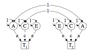
There are different ways to draw a path diagram of the ACE model. The most commonly used approach is with the three latent variables in circles at the top, separately for twin 1 and twin 2 respectively called A1, C1, E1 and A2, C2, E2. The latent variables are connected to the observed variables (in boxes) *bmi1* and *bmi2* at the bottom by single-headed arrows from the latent to the manifest variables. Path coefficients a, c and e are estimated but constrained to be the same for twin 1 and twin 2, as well as for MZ and DZ twins. As MZ twins share all their genotypes, the double-headed path connecting A1 and A2 is fixed to one. DZ twins share on average half their genes, as a result the corresponding path is fixed to 0.5 in the DZ diagram. As environmental factors that are shared between twins are assumed to increase similarity between twin to the same extent in MZ and DZ twins (equal environments assumption), the double-headed path connecting C1 and C2 is fixed to one in both diagrams. The unique environmental factors are by definition uncorrelated between twins.

Let’s go through each of the paths specification step by step. They will all form arguments of the mxModel, specified as follows. Given the diagrams for the MZ and the DZ group look rather similar, we start by specifying all the common elements which will then be shared with the two submodels for each of the twin types. Thus we call the first model ‘share’.

#Fit ACE Model with RawData and Path-style Input
share <- mxModel("share",
    type="RAM",

Models specifying paths are translated into ‘RAM’ specifications for optimization, indicated by using the type='RAM'. For further details on RAM, see ref. Note that we left the comma’s at the end of the lines which are necessary when all the arguments are combined prior to running the model. Each line can be pasted into R, and then evaluated together once the whole model is specified. We start the path diagram specification by providing the names for the manifest variables in manifestVars and the latent varibles in latentVars. We use here the ‘selVars’ and ‘aceVars’ objects that we created before when preparing the data.

manifestVars=selVars,
latentVars=aceVars,

We start by specifying paths for the variances and means of the latent variables. This includes double-headed arrows from each latent variable back to itself, fixed at one, and single-headed arrows from the triangle (with a fixed value of one) to each of the latent variables, fixed at zero. Next we specify paths for the means of the observed variables using single-headed arrows from ‘one’ to each of the manifest variables. These are set to be free and given a start value of 20. As we use the same label (“mean”) for the two means, they are constrained to be equal. The main paths of interest are those from each of the latent variables to the respective observed variable. These are also estimated (thus all are set free), get a start value of .6 and appropriate labels. As the common environmental factors are by definition the same for both twins, we fix the correlation between C1 and **C2 to one.

mxPath(
    from=aceVars,
    arrows=2,
    free=FALSE,
    values=1
),
mxPath(
    from="one",
    to=aceVars,
    arrows=1,
    free=FALSE,
    values=0
),
mxPath(
    from="one",
    to=selVars,
    arrows=1, free=TRUE,
    values=20,
    labels= c("mean","mean")
),
mxPath(
    from=c("A1","C1","E1"),
    to="bmi1",
    arrows=1,
    free=TRUE,
    values=.6,
    label=c("a","c","e")
),
mxPath(
    from=c("A2","C2","E2"),
    to="bmi2",
    arrows=1,
    free=TRUE,
    values=.6,
    label=c("a","c","e")
),
mxPath(
    from="C1", to="C2",
    arrows=2,
    free=FALSE,
    values=1
)
)

We add the paths that are specific to the MZ group or the DZ group into the respective submodels which will be combined in ‘twinACEModel’. So we have two mxModel statement within the “twinACE” model statement. Each of the two models are based on the previously specified “share” model by including it as its first argument. Then we add the path for the correlation between A1 and A2 which is fixed to one for the MZ group. That concludes the specification of the model for the MZ’s, thus we move to the mxData command that calls up the data.frame with the MZ raw data, with the type specified explicitly. Given we use the path specification, the objective function uses RAM, thus type='RAM'. We also give it the model a name to refer back to it later when we need to add the objective functions. The mxModel command for the DZ group is very similar, except that the the correlation between A1 and A2 is fixed to 0.5 and the DZ data are read in.

twinACEModel <- mxModel("twinACE",
    mxModel(share,
        mxPath(
            from="A1",
            to="A2",
            arrows=2,
            free=FALSE,
            values=1
        ),
        mxData(
            observed=mzfData,
            type="raw"),
        type="RAM",
        name="MZ"
    ),
    mxModel(share,
        mxPath(
            from="A1",
            to="A2",
            arrows=2,
            free=FALSE,
            values=.5
        ),
        mxData(
            observed=dzfData,
            type="raw"
        ),
        type="RAM",
        name="DZ"
    ),

Finally, both models need to be evaluated simultaneously. We first generate the sum of the objective functions for the two groups, using mxAlgebra, and then use that as argument of the mxAlgebraObjective command.

    mxAlgebra(
        expression=MZ.objective + DZ.objective,
        name="twin"
    ),
    mxAlgebraObjective("twin")
)

Model Fitting¶

We need to invoke the mxRun command to start the model evaluation and optimization. Detailed output will be available in the resulting object, which can be obtained by a print() statement.

#Run ACE model
twinACEFit <- mxRun(twinACEModel)

Often, however, one is interested in specific parts of the output. In the case of twin modeling, we typically will inspect the expected covariance matrices and mean vectors, the parameter estimates, and possibly some derived quantities, such as the standardized variance components, obtained by dividing each of the components by the total variance. Note in the code below that the mxEvaluate command allows easy extraction of the values in the various matrices/algebras which form the first argument, with the model name as second argument. Once these values have been put in new objects, we can use and regular R expression to derive further quantities or organize them in a convenient format for including in tables. Note that helper functions could (and will likely) easily be written for standard models to produce ‘standard’ output.

MZc <- mxEvaluate(MZ.covariance, twinACEFit)
DZc <- mxEvaluate(DZ.covariance, twinACEFit)
M <- mxEvaluate(MZ.means, twinACEFit)
A <- mxEvaluate(a*a, twinACEFit)
C <- mxEvaluate(c*c, twinACEFit)
E <- mxEvaluate(e*e, twinACEFit)
V <- (A+C+E)
a2 <- A/V
c2 <- C/V
e2 <- E/V
ACEest <- rbind(cbind(A,C,E),cbind(a2,c2,e2))
LL_ACE <- mxEvaluate(objective, twinACEFit)

Alternative Models: an AE Model¶

To evaluate the significance of each of the model parameters, nested submodels are fit in which these parameters are fixed to zero. If the likelihood ratio test between the two models is significant, the parameter that is dropped from the model significantly contributes to the phenotype in question. Here we show how we can fit the AE model as a submodel with a change in two mxPath commands. First, we call up the previous ‘full’ model and save it as a new model ‘twinAEModel’. Next we re-specify the path from C1 to bmi1 to be fixed to zero, and do the same for the path from C2 to bmi2. We can run this model in the same way as before and generate similar summaries of the results.

#Run AE model
twinAEModel <- mxModel(twinACEModel,
    type="RAM",
    manifestVars=selVars,
    latentVars=aceVars,
    mxPath(
        from=c("A1","C1","E1"),
        to="bmi1",
        arrows=1,
        free=c(T,F,T),
        values=c(.6,0,.6),
        label=c("a","c","e")
    ),
    mxPath(
        from=c("A2","C2","E2"),
        to="bmi2",
        arrows=1,
        free=c(T,F,T),
        values=c(.6,0,.6),
        label=c("a","c","e")
    )
)
twinAEFit <- mxRun(twinAEModel)

MZc <- mxEvaluate(MZ.covariance, twinAEFit)
DZc <- mxEvaluate(DZ.covariance, twinAEFit)
M <- mxEvaluate(MZ.means, twinAEFit)
A <- mxEvaluate(a*a, twinAEFit)
C <- mxEvaluate(c*c, twinAEFit)
E <- mxEvaluate(e*e, twinAEFit)
V <- (A + C + E)
a2 <- A / V
c2 <- C / V
e2 <- E / V
AEest <- rbind(cbind(A, C, E),cbind(a2, c2, e2))
LL_AE <- mxEvaluate(objective, twinAEFit)

We use a likelihood ratio test (or take the difference between -2 times the log-likelihoods of the two models) to determine the best fitting model, and print relevant output.

LRT_ACE_AE <- LL_AE - LL_ACE

#Print relevant output
ACEest
AEest
LRT_ACE_AE

Definition Variables, Path Specification¶

This example will demonstrate the use of OpenMx definition variables with the analysis of a simple two group dataset. What are definition variables? Essentially, definition variables can be thought of as observed variables that are used to change the statistical model on an individual case basis. In essence, it is as though one or more variables in the raw data vectors are used to specify the statistical model for that individual. Many different types of statistical model can be specified in this fashion; some are readily specified in standard fashion, and some cannot. To illustrate, we implement a two-group model. The groups differ in their means but not in their variances and covariances. This situation could easily be modeled in a regular multiple group fashion - it is only implemented using definition variables to illustrate their use. The results are verified using summary statistics and an Mx 1.0 script for comparison is also available.

Mean Differences¶

The scripts are presented here

DefinitionMeans_PathRaw.R
DefinitionMeans_PathRaw.mx

Statistical Model¶

Algebraically, we are going to fit the following model to the observed x and y variables:

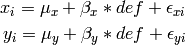
$\begin{eqnarray*} x_{i} = \mu_{x} + \beta_x * def + \epsilon_{xi}\\ y_{i} = \mu_{y} + \beta_y * def + \epsilon_{yi} \end{eqnarray*}$

where the residual sources of variance, $\epsilon_{xi}$ and $\epsilon_{yi}$ covary to the extent $\rho$ . So, the task is to estimate: the two means $\mu_{x}$ and $\mu_{y}$ ; the deviations from these means due to belonging to the group identified by having def set to 1 (as opposed to zero), $\beta_{x}$ and $\beta_{y}$ ; and the parameters of the variance covariance matrix: cov( $\epsilon_{x},\epsilon_{y}$ ).

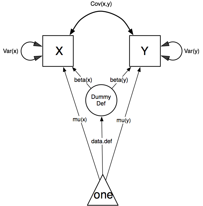
Our task is to implement the model shown in the Figure below:

Data Simulation¶

Our first step to running this model is to simulate the data to be analyzed. Each individual is measured on two observed variables, x and y, and a third variable “def” which denotes their group membership with a 1 or a 0. These values for group membership are not accidental, and must be adhered to in order to obtain readily interpretable results. Other values such as 1 and 2 would yield the same model fit, but would make the interpretation more difficult.

library(MASS)  # to get hold of mvrnorm function

set.seed(200)  # to make the simulation repeatable
n = 500        # sample size, per group

Sigma <- matrix(c(1,.5,.5,1),2,2)
group1<-mvrnorm(n=n, c(1,2), Sigma)
group2<-mvrnorm(n=n, c(0,0), Sigma)

We make use of the superb R function mvrnorm in order to simulate n=500 records of data for each group. These observations correlate .5 and have a variance of 1, per the matrix Sigma. The means of x and y in group 1 are 1.0 and 2.0, respectively; those in group 2 are both zero. The output of the mvrnorm function calls are matrices with 500 rows and 3 columns, which are stored in group 1 and group 2. Now we create the definition variable

# Put the two groups together, create a definition variable,
# and make a list of which variables are to be analyzed (selvars)
y<-rbind(group1,group2)
dimnames(y)[2]<-list(c("x","y"))
def<-rep(c(1,0),each=n)
selvars<-c("x","y")

The objects y and def might be combined in a data frame. However, in this case we won’t bother to do it externally, and simply paste them together in the mxData function call.

Model Specification¶

Before specifying a model, the OpenMx library must be loaded into R using either the require() or library() function. This code uses the mxModel function to create an mxModel object, which we’ll then run. Note that all the objects required for estimation (data, matrices, and an objective function) are declared within the mxModel function. This type of code structure is recommended for OpenMx scripts generally.

require(OpenMx)
defmeansmodel<-mxModel("Definition Means via Paths",
    type="RAM",

The first argument in an mxModel function has a special function. If an object or variable containing an MxModel object is placed here, then mxModel adds to or removes pieces from that model. If a character string (as indicated by double quotes) is placed first, then that becomes the name of the model. Models may also be named by including a name argument. This model is named "DefinitionMeans".

The second line of the mxModel function call declares that we are going to be using RAM specification of the model, using directional and bidirectional path coefficients between the variables. Next, we declare where the data are, and their type, by creating an MxData object with the mxData function. This code first references the object where our data are, then uses the type argument to specify that this is raw data. Analyses using definition variables have to use raw data, so that the model can be specified on an individual data vector level.

mxData(
    observed=data.frame(y,def),
    type="raw"),
manifestVars=c("x","y"),
latentVars="DefDummy",

Model specification is carried out using two lists of variables, manifestVars and latentVars. Then mxPath functions are used to specify paths between them. In the present case, we need four mxPath commands to specify the model. The first is for the variances of the x and y variables, and the second specifies their covariance. The third specifies a path from the mean vector, always known by the special keword “one”, to each of the observed variables, and to the single latent variable “DefDummy”. This last path is specified to contain the definition variable, by virtue of the “data.def” label. Finally, two paths are specified from the “DefDummy” latent variable to the observed variables. These parameters estimate the deviation of the mean of those with a data.def value of 1 from that of those with data.def values of zero.

mxPath(from=c("x","y"),
    arrows=2,
    free=TRUE,
    values=c(1,.1,1),
    labels=c("Varx","Vary")
), # variances
mxPath(from="x", to="y",
    arrows=2,
    free=TRUE,
    values=c(.1),
    labels=c("Covxy")
), # covariances
mxPath(from="one",
    to=c("x","y","DefDummy"),
    arrows=1,
    free=c(TRUE,TRUE,FALSE),
    values=c(1,1,1),
    labels =c("meanx","meany","data.def")
), # means
mxPath(from="DefDummy",
    to=c("x","y"),
    arrows=1,
    free=c(TRUE,TRUE),
    values=c(1,1),
    labels =c("beta_1","beta_2")
) # moderator paths

)

We can then run the model and examine the output with a few simple commands.

Model Fitting¶

# Run the model
defMeansFit<-mxRun(defMeansModel)
defMeansFit@matrices

The R object defmeansresult contains matrices and algebras; here we are interested in the matrices, which can be seen with the defmeansresult@matrices entry. In path notation, the unidirectional, one-headed arrows appear in the matrix A, the two-headed arrows in S, and the mean vector single headed arrows in M.

# Compare OpenMx estimates to summary statistics from raw data,
# remembering to knock off 1 and 2 from group 1's data
# so as to estimate variance of combined sample without
# the mean difference contributing to the variance estimate.

# First we compute some summary statistics from the data
ObsCovs <- cov(rbind(group1 - rep(c(1,2), each=n), group2))
ObsMeansGroup1 <- c(mean(group1[,1]), mean(group1[,2]))
ObsMeansGroup2 <- c(mean(group2[,1]), mean(group2[,2]))

# Second we extract the parameter estimates and matrix algebra results from the model
Sigma<-defmeansresult@matrices$S@values[1:2,1:2]
Mu<-defmeansresult@matrices$M@values[1:2]
beta<-defmeansresult@matrices$A@values[1:2,3]

# Third, we check to see if things are more or less equal
omxCheckCloseEnough(ObsCovs,Sigma,.01)
omxCheckCloseEnough(ObsMeansGroup1,as.vector(Mu+beta),.001)
omxCheckCloseEnough(ObsMeansGroup2,as.vector(Mu),.001)

Navigation

Examples, Path Specification¶

Regression, Path Specification¶

Simple Regression¶

Data¶

Model Specification¶

Model Fitting¶

Multiple Regression¶

Multivariate Regression¶

Factor Analysis, Path Specification¶

Common Factor Model¶

Data¶

Model Specification¶

Two Factor Model¶

Time Series, Path Specification¶

Latent Growth Curve Model¶

Data¶

Model Specification¶

Multiple Groups, Path Specification¶

Heterogeneity Model¶

Data¶

Model Specification¶

Model Fitting¶

Homogeneity Model: a Submodel¶

Model Specification¶

Model Fitting¶

Genetic Epidemiology, Path Specification¶

ACE Model: a Twin Analysis¶

Data¶

Model Specification¶

Model Fitting¶

Alternative Models: an AE Model¶

Definition Variables, Path Specification¶

Mean Differences¶

Statistical Model¶

Data Simulation¶

Model Specification¶

Model Fitting¶

Table Of Contents

Previous topic

Next topic

This Page

Quick search

Navigation